Library Examples (libHYPREDRV)

This section demonstrates how to use the libHYPREDRV library from application codes that assemble their own linear systems. Unlike the Driver Examples (hypredrive-cli), which drive the hypredrive-cli executable from YAML input files and file-based matrix/RHS data, these examples embed the matrix/vector assembly directly in the application. This is the right mode when the application owns the discretization, data layout, MPI partitioning, and solver lifecycle, but still wants hypredrive to configure and invoke HYPRE solvers and preconditioners.

Note

Prefer the hypredrive-cli driver when working with matrices/vectors on disk or when quickly comparing solver/preconditioner configurations. Prefer libHYPREDRV when your application assembles matrices and vectors in memory and needs a lightweight API to invoke HYPRE programmatically.

Examples at a Glance

Click any panel (image or title) to jump to the full example.

1. Laplace’s equation	2. Mixed Darcy Flow	3. Linear Elasticity
4. Nonlinear Heat Flow	5. Navier-Stokes	6. Definite curl-curl (AMS)
7. Definite grad-div (ADS)

Overview of Typical Steps

Note

This section focuses on the C/C++ library API. For language bindings, see Interfaces, especially Python Interface and Fortran Interface.

The library-side workflow in C/C++ generally follows these steps:

1. Initialize MPI (if not already done).

2. Initialize hypredrive and create an object handle.

3. Call HYPREDRV_SetLibraryMode to signal library use (must precede step 4).

4. Parse a YAML configuration string/file to set solver/preconditioner options.

5. Assemble your matrix and vectors (HYPRE_IJMatrix/HYPRE_IJVector) in parallel.

6. Tell hypredrive about your DOF layout (e.g., interleaved blocks).

7. Attach matrix/RHS/initial guess/prec matrix to hypredrive.

8. Create, set up, apply, and destroy the solver.

9. Retrieve host-accessible solution values or statistics if needed. In library mode, general.statistics is flushed automatically when the HYPREDRV_t object is destroyed; call HYPREDRV_StatsPrint only if you want an earlier snapshot. Set general.statistics_filename to append summaries to a file instead of stdout.

10. Destroy handles explicitly when practical, then finalize hypredrive. HYPREDRV_Finalize() auto-destroys any remaining live handles, but it cannot rewrite your local handle variables to NULL.

If you manage multiple handles, set general.name in YAML or call HYPREDRV_ObjectSetName so statistics can identify which object produced each summary.

If your application owns multiple HYPREDRV_t objects concurrently, or if you want preconditioner reuse to respect application-defined timestep / nonlinear-iteration boundaries, use the annotation APIs (HYPREDRV_AnnotateBegin / HYPREDRV_AnnotateEnd and HYPREDRV_AnnotateLevelBegin / HYPREDRV_AnnotateLevelEnd).

A minimal skeleton of a program using the library is shown below.

#include "HYPREDRV.h"
#include <mpi.h>

int main(int argc, char** argv) {
  MPI_Init(&argc, &argv);

  HYPREDRV_t h;
  HYPREDRV_Initialize();
  HYPREDRV_Create(MPI_COMM_WORLD, &h);

  // Signal that this is a library-mode caller (must precede InputArgsParse)
  HYPREDRV_SetLibraryMode(h);
  HYPREDRV_ObjectSetName(h, "flow-solver");

  // Provide YAML configuration
  const char* yaml = "general:\n"
                     "  statistics: 1\n"
                     "  statistics_filename: stats.txt\n"
                     "solver:\n"
                     "  pcg: {}\n"
                     "preconditioner:\n"
                     "  amg: {}\n";
  char* args[1] = {(char*)yaml};
  HYPREDRV_InputArgsParse(1, args, h);

  // Build IJ objects (global row range per rank) and assemble your system
  HYPRE_IJMatrix A;
  HYPRE_IJVector b;
  /* ... create/initialize/insert/assemble A, b ... */

  // Set linear system components
  HYPREDRV_LinearSystemSetMatrix(h, (HYPRE_Matrix)A);
  HYPREDRV_LinearSystemSetRHS(h, (HYPRE_Vector)b);
  HYPREDRV_LinearSystemSetInitialGuess(h, NULL);
  HYPREDRV_LinearSystemSetReferenceSolution(h, NULL);
  HYPREDRV_LinearSystemSetPrecMatrix(h, NULL);

  // Solve lifecycle
  HYPREDRV_LinearSolverCreate(h);
  HYPREDRV_LinearSolverSetup(h);
  HYPREDRV_LinearSolverApply(h);
  HYPREDRV_LinearSolverDestroy(h);

  // (Optional) Query statistics early and retrieve host solution values
  // (general.statistics also prints automatically on destroy in library mode)
  HYPREDRV_StatsPrint(h);
  HYPRE_Real* xvals = NULL;
  HYPREDRV_LinearSystemGetSolutionValues(h, &xvals);

  // Cleanup
  HYPRE_IJMatrixDestroy(A);
  HYPRE_IJVectorDestroy(b);
  HYPREDRV_Destroy(&h);
  HYPREDRV_Finalize();
  MPI_Finalize();
  return 0;
}

• YAML configuration can be provided as an in-memory string (as shown above, where the char* is passed directly as argv[0]) or as a path to a ``.yml`` / ``.yaml`` file on disk. The YAML structure is identical in both cases.

• For block linear systems, set row mapping information via HYPREDRV_LinearSystemSetDofmap.

• If compiled with GPU support, you may migrate assembled IJ objects to device memory with HYPRE_IJMatrixMigrate(..., HYPRE_MEMORY_DEVICE) and analogous calls for vectors.

• HYPREDRV_LinearSystemSetInitialGuess, HYPREDRV_LinearSystemSetReferenceSolution, and HYPREDRV_LinearSystemSetPrecMatrix accept optional external vectors/matrix. Passing NULL asks hypredrive to use the configured/default behavior. Passing non-NULL uses the provided object.

• Ownership follows library mode. After HYPREDRV_SetLibraryMode, non-NULL HYPRE objects supplied by the caller are borrowed and remain caller-owned. Without library mode, non-NULL objects passed through these setters are treated as hypredrive-owned and destroyed with the HYPREDRV_t object.

Note

Preconditioner reuse across a sequence of linear systems (time steps, multiple RHS) is configured via the preconditioner.reuse YAML subsection. See Preconditioner reuse in the Input Structure (YAML) reference. In embedded multi-handle applications, drive timestep boundaries with HYPREDRV_AnnotateLevelBegin / HYPREDRV_AnnotateLevelEnd so reuse decisions stay attached to the correct HYPREDRV_t object.

For example, an embedded caller that wants reuse to restart at each timestep can bracket the solve lifecycle like this:

HYPREDRV_AnnotateLevelBegin(h, 0, "timestep-7", -1);
HYPREDRV_AnnotateLevelBegin(h, 1, "newton-0", -1);
HYPREDRV_AnnotateBegin(h, "system", -1);
HYPREDRV_LinearSolverCreate(h);
HYPREDRV_LinearSolverSetup(h);
HYPREDRV_AnnotateEnd(h, "system", -1);
HYPREDRV_LinearSolverApply(h);
HYPREDRV_AnnotateLevelEnd(h, 1, "newton-0", -1);
HYPREDRV_AnnotateLevelEnd(h, 0, "timestep-7", -1);

You can also select a predefined preconditioner preset programmatically, without a YAML file:

HYPREDRV_SetLibraryMode(h);
HYPREDRV_InputArgsSetPreconPreset(h, "poisson");

If you subsequently call HYPREDRV_InputArgsParse with a YAML string or file, the parsed YAML settings will override the preset for any keys it defines.

Example 1: Laplace’s equation

This section documents a scalar diffusion/Laplace example assembled directly from an application using the hypre IJ interface via libHYPREDRV. It mirrors the driver in examples/src/C_laplacian/laplacian.c and demonstrates multiple finite-difference stencils on a structured grid.

Governing equation and boundary conditions

We solve

\[\begin{split}-\nabla\!\cdot\!\big(\mathbf{c}\,\nabla u\big) \;=\; 0 \quad \text{in } \Omega=[0,1]^3, \\ u \;=\; 0 \ \text{on } \partial\Omega\setminus\{y=0\},\\ u \;=\; 1 \ \text{on } \{y=0\}\end{split}\]

Anisotropy is supported through directional coefficients (see below). A pure Dirichlet setup yields a symmetric positive definite (SPD) linear system. We discretize on a uniform structured grid with global node counts \(N=(N_x,N_y,N_z)\) and spacings \(h_x = 1/(N_x-1)\), \(h_y = 1/(N_y-1)\), \(h_z = 1/(N_z-1)\). Nodes are indexed lexicographically with \(x\) fastest. Parallel partitioning uses an MPI Cartesian grid \(P=(P_x,P_y,P_z)\) with block starts pstarts[d].

Finite-difference stencils

We support several stencils for \(-\nabla\!\cdot(\mathbf{c}\nabla u)\) on a structured grid. All produce an M-matrix (positive diagonal, non-positive off-diagonals) and are second-order accurate when weights are chosen consistently.

7-point (faces only, classical 2nd order)

With directional coefficients \(c_x,c_y,c_z\) and spacings \(h_x,h_y,h_z\), the discrete negative-Laplacian operator at interior node \((i,j,k)\) is

\[\begin{split}\begin{aligned} (A_h u)_{i,j,k} &= \frac{c_x}{h_x^2}\,\big(2u_{i,j,k} - u_{i+1,j,k} - u_{i-1,j,k}\big) + \\ &\quad \frac{c_y}{h_y^2}\,\big(2u_{i,j,k} - u_{i,j+1,k} - u_{i,j-1,k}\big) + \\ &\quad \frac{c_z}{h_z^2}\,\big(2u_{i,j,k} - u_{i,j,k+1} - u_{i,j,k-1}\big) \end{aligned}\end{split}\]

19-point (faces + edges)

Adds edge neighbors (e.g., \((i\pm1,j\pm1,k)\), etc.) with scaled couplings to reduce directional bias. A common strategy is to assign edge weights that partially compensate cross-term truncation errors from a Taylor expansion, while preserving diagonal dominance and the M-matrix structure.

27-point (faces + edges + corners)

Includes the full \(3\times3\times3\) neighborhood (faces, edges, corners). Corner weights are smaller than faces; one can tune edge/corner weights (e.g., half/third of face weights) to further reduce dispersion and directional bias.

125-point (radius-2 demo)

Extends the neighborhood to radius 2 (up to 125 points). In the example driver, face-adjacent neighbors often receive stronger weights (e.g., \(-1\)), while farther neighbors receive smaller negative weights (e.g., \(-0.01\)), preserving an M-matrix with a dominant diagonal.

Coefficients and anisotropy

The example exposes coefficient arrays in the driver (params->c). For 7-point, only face-connected neighbors are used with directional weights, e.g., in dimension-wise form

\[(A u)_{i,j,k} \;\approx\; \sum_{\alpha\in\{x,y,z\}} \frac{c_\alpha}{h_\alpha^2}\,\big(-u_{i-\hat\alpha} + 2u_{i} - u_{i+\hat\alpha}\big).\]

For 19/27-point, the example scales edge/corner couplings (e.g., half/third) to reduce cross terms, preserving a strictly diagonally dominant M-matrix. The 125-point variant uses uniform small weights for far neighbors to illustrate wide stencils.

Boundary Conditions and SPD Structure

Dirichlet values are enforced during assembly. When a neighbor lies outside \(\Omega\), or when the face corresponds to \(y=0\) with \(u=1\), the known-value contribution is moved to the RHS. Rows for interior nodes use only valid neighbor columns; the diagonal entry is the negative sum of off-diagonals to maintain row-sum consistency and the SPD structure.

Linear System Creation (IJ interface)

• Create HYPRE_IJMatrix/HYPRE_IJVector on the Cartesian communicator with global row range [ilower, iupper] for this rank.

• Set per-row nnz bounds according to the stencil (7, 19, 27, 125) with HYPRE_IJMatrixSetRowSizes; initialize IJ objects.

• For each local node, compute the global row (block-aware), enumerate stencil neighbors, and build column/value arrays. Off-partition neighbors remain valid columns (IJ distributes); out-of-domain neighbors contribute to the RHS via Dirichlet handling above.

• Insert with HYPRE_IJMatrixSetValues (or AddToValues) and HYPRE_IJVectorSetValues, then assemble.

This is a scalar problem (one DOF per node), so no interleaved dofmap is required before attaching the matrix/vector to hypredrive.

Linear Solver Setup

Solver and preconditioner options (PCG+AMG by default) are provided via YAML parsed with HYPREDRV_InputArgsParse; the create/setup/apply sequence honors those settings.

// After building IJ A,b as a scalar system:
HYPREDRV_LinearSystemSetMatrix(hdrv, (HYPRE_Matrix)A);
HYPREDRV_LinearSystemSetRHS(hdrv,    (HYPRE_Vector)b);
HYPREDRV_LinearSystemSetInitialGuess(hdrv, NULL);   // zero by default
HYPREDRV_LinearSystemSetPrecMatrix(hdrv, NULL);     // reuse A if desired

// Solve lifecycle
HYPREDRV_LinearSolverCreate(hdrv);
HYPREDRV_LinearSolverSetup(hdrv);
HYPREDRV_LinearSolverApply(hdrv);
HYPREDRV_LinearSolverDestroy(hdrv);

The default in the example is a conjugate gradient solver with a BoomerAMG preconditioner. Additional AMG parameters (e.g., coarsening, interpolation) can be specified as needed in the YAML configuration.

Visualizing the Solution

With -vis the example writes the solution as VTK RectilinearGrid – a per-rank .vtr plus a .pvd collection – with the scalar point field solution. Ghost exchanges (faces/edges/corners) assemble an overlapped piece on negative faces to avoid cracks at partition boundaries. The bundled postprocess.py renders the field with PyVista; by default it draws nested translucent isosurfaces (--style also offers clip, volume, and slices), matching the Maxwell and grad-div examples:

mpirun -np 4 /path/to/build/laplacian -n 65 65 65 -P 2 2 1 -vis
python3 postprocess.py laplacian_7pt_65x65x65_2x2x1.pvd -o laplacian_solution_3d.png   # needs: pip install pyvista

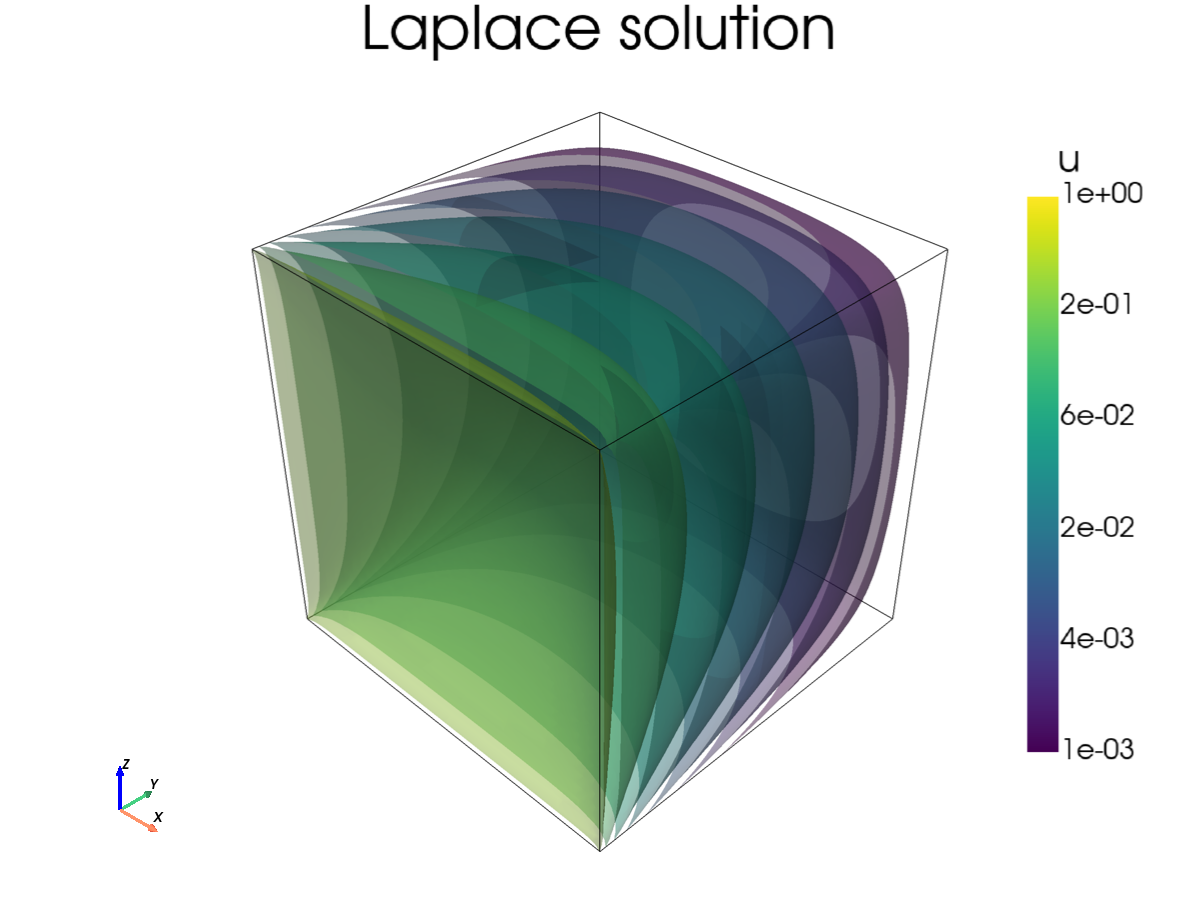
Solution \(u\) on a \(64^3\) grid, shown as nested isosurfaces with a logarithmic color scale. The Dirichlet datum \(u=1\) on the \(y=0\) face diffuses into the domain and decays by orders of magnitude toward the far boundaries. The same .pvd/.vtr files can also be opened directly in ParaView.

Reproducible Run

Command-line parameters (see laplacian -h) control problem size, coefficients, partitioning, number of solves, printing, verbosity, and visualization.

mpirun -np 1 /path/to/build/examples/src/C_laplacian/laplacian -h

Usage: ${MPIEXEC_COMMAND} ${MPIEXEC_NUMPROC_FLAG} <np> ./laplacian [options]

Options:
  -i <file>         : YAML configuration file for solver settings
  -n <nx> <ny> <nz> : Global grid dimensions (default: 10 10 10)
  -c <cx> <cy> <cz> : Diffusion coefficients (default: 1.0 1.0 1.0)
  -P <Px> <Py> <Pz> : Processor grid dimensions (default: 1 1 1)
  -s <val>          : Stencil type: 7 19 27 125 (default: 7)
  -ns|--nsolve <n>  : Number of times to solve the system (default: 5)
  -vis|--visualize  : Output solution in VTK format (default: false)
  -p|--print        : Print matrices/vectors to file (default: false)
  -v|--verbose <n>  : Verbosity level (bitset):
                      0x1: Print solver statistics
                      0x2: Print library info
                      0x4: Print system info
  -h|--help         : Print this message

For a single-process run, the output should be similar to the following:

mpirun -np 1 /path/to/build/examples/src/C_laplacian/laplacian

Date and time: YYYY-MM-DD HH:MM:SS

Using HYPREDRV_DEVELOP_STRING: HYPREDRV_VERSION_GOES_HERE

Running on 1 MPI rank

=====================================================
              Laplacian Problem Setup
=====================================================
Grid dimensions:      10 x 10 x 10
Processor topology:   1 x 1 x 1
Diffusion coeffs:     (1.00e+00, 1.00e+00, 1.00e+00)
Discretization:       7-point stencil
Visualization:        false
Verbosity level:      0x3
Number of solves:     5
=====================================================

Assembling linear system... Done!
Solve 1/5...
Solve 2/5...
Solve 3/5...
Solve 4/5...
Solve 5/5...
====================================================================================


STATISTICS SUMMARY:

+--------+-------------+-------------+-------------+------------+------------+--------+
|        |    LS build |       setup |       solve |    initial |   relative |        |
|  Entry |   times [s] |   times [s] |   times [s] |  res. norm |  res. norm |  iters |
+--------+-------------+-------------+-------------+------------+------------+--------+
|      0 |       0.008 |       0.001 |       0.000 |   1.00e+01 |   6.12e-07 |      5 |
|      1 |             |       0.001 |       0.000 |   1.00e+01 |   6.12e-07 |      5 |
|      2 |             |       0.001 |       0.000 |   1.00e+01 |   6.12e-07 |      5 |
|      3 |             |       0.001 |       0.000 |   1.00e+01 |   6.12e-07 |      5 |
|      4 |             |       0.001 |       0.000 |   1.00e+01 |   6.12e-07 |      5 |
+--------+-------------+-------------+-------------+------------+------------+--------+

Date and time: YYYY-MM-DD HH:MM:SS
/home/victor/projects/hypredrive-master/build-v3.0.0/laplacian done!

Note

Python examples live under interfaces/python/examples; see Python Interface. The Fortran Laplacian example lives under interfaces/fortran/examples/laplacian; see Fortran Interface.

Example 2: Mixed Darcy Flow

This section documents the mixed Darcy driver implemented in examples/src/C_darcy/darcy.c. The example uses the standard C libHYPREDRV interface: the application assembles HYPRE_IJMatrix and HYPRE_IJVector objects, supplies a dofmap, and lets hypredrive configure GMRES with an MGR preconditioner. The current implementation provides an RT0/P0 discretization descriptor; the assembly is organized so future mixed discretizations can replace the cell-local flux dofs and mass entries without changing the solver interface.

Governing Equations

On a Cartesian domain \(\Omega=[0,L_x]\times[0,L_y]\times[0,L_z]\), Darcy flow is written in mixed first-order form

\[\mathbf{q} + K\nabla u = 0,\qquad \nabla\!\cdot\mathbf{q} = f,\]

with pressure \(u\), flux \(\mathbf{q}\), permeability tensor \(K\), Dirichlet pressure data on \(\Gamma_D\), and prescribed normal flux on \(\Gamma_N\). The example uses f=0 and supports diagonal permeability fields, either constant over the domain or read as per-cell heterogeneous values. By default it imposes a unit pressure drop along the selected active axis: \(u=1\) on the low boundary, \(u=0\) on the high boundary, and no-flow boundaries on the remaining active axes.

RT0/P0 Discretization

The implemented discretization uses lowest-order Raviart–Thomas fluxes (RT0) and cellwise constant pressures (P0). One pressure unknown is stored per cell. Flux unknowns live on mesh faces and represent integrated normal flux

\[q_F = \int_F \mathbf{q}\cdot\mathbf{n}_F\,dS,\]

where \(\mathbf{n}_F\) is the global positive coordinate normal of that face. For a cell \(K_c\), the local mixed blocks are

\[\begin{split}M_{ab}^{(c)} = (K^{-1})_{d_a d_b}\,|K_c|\,\frac{\alpha_{ab}}{|F_a|\,|F_b|}, \qquad B_{a,c}=\begin{cases} -1 & F_a \text{ is the low face of } K_c,\\ +1 & F_a \text{ is the high face of } K_c, \end{cases}\end{split}\]

where \(d_a\) is the coordinate direction of local face \(F_a\). For diagonal permeability, only same-direction face pairs contribute. The RT0 mass block uses \(\alpha_{ab}=1/3\) for same-direction same-side faces and \(\alpha_{ab}=1/6\) for same-direction opposite-side faces.

After negating the continuity equation to get the symmetric saddle-point sign convention before boundary row pinning, the global system is

\[\begin{split}\begin{bmatrix} M & -B\\ -B^T & 0 \end{bmatrix} \begin{bmatrix} \mathbf{q}\\ \mathbf{u} \end{bmatrix} = \begin{bmatrix} \mathbf{g}_D\\ 0 \end{bmatrix}.\end{split}\]

Dirichlet pressure data enters the flux equations through \(-\int_{\Gamma_D}u_D\,\mathbf{v}\cdot\mathbf{n}_{out}\,dS\). No-flow Neumann faces are enforced as zero-valued pinned flux rows. Since the pinned value is zero, the example leaves columns intact; this is parallel-safe for an IJ row-partitioned assembly and preserves the intended solution.

Parallel Numbering and C Interface Assembly

The C example uses a rank-contiguous global unknown ordering. Within each rank, owned unknowns are ordered

\[[\,x\text{-faces}\,][\,y\text{-faces}\,][\,z\text{-faces}\,][\,cells\,],\]

with inactive face blocks omitted for 1D/2D prefix-active meshes. The Cartesian rank grid is selected automatically by default and can be set explicitly with -P/--procs <px> <py> <pz>. The product must match the MPI size, and inactive dimensions must have partition count 1.

Faces are owned by the rank on their high-coordinate side, with the global high boundary face owned by the last rank in that direction. Cells are owned by their Cartesian subdomain. Each rank builds a local CSR slab over its contiguous row range and passes it to hypredrive, with off-rank columns left as global column indices.

The dofmap is supplied explicitly:

• label 1 for flux-face rows,

• label 0 for cell-pressure rows.

This is intentionally independent of the RT0 cell-local helper. A higher-order mixed method can keep the same solver-facing labels while replacing the discretization descriptor that enumerates cell dofs and local matrices.

Heterogeneous Permeability Files

The -K option sets a constant diagonal permeability \((K_x,K_y,K_z)\). Alternatively, --K-file reads a whitespace-delimited text file containing either one scalar permeability per source cell or three component blocks Kx, Ky, and Kz. If --K-file-grid is omitted, the source grid is assumed to match -n exactly. If a source grid is supplied, the example samples the source field at cell centers onto the requested mesh. This is useful for experiments on a coarser mesh than the input data, for refinement studies across a sequence of mesh resolutions, and for mesh-sequence scalability measurements.

SPE10 model 2 permeability files use a 60 x 220 x 85 source grid with three component blocks. The helper script downloads and unpacks that dataset into an ignored directory:

scripts/download_spe10_case2a.sh

Then run a coarse heterogeneous solve, for example:

mpirun -np 2 /path/to/build/darcy -n 8 8 4 \
   -P 1 1 2 \
   --K-file data/spe10_case2a/spe_perm.dat \
   --K-file-grid 60 220 85 \
   --K-file-k-order top-down \
   -g y -v 0

The -g y option imposes the pressure gradient in the y-direction, which is the standard SPE10 setup.

For heterogeneous inputs, the driver reports successful solver completion rather than an analytic pressure error because the default linear pressure profile is no longer the exact solution.

SPE10 Reproduction Script

The C Darcy example directory includes a reproducibility script for the SPE10 case:

examples/src/C_darcy/reproduce.sh

By default, the script downloads the ignored SPE10 data if needed, builds the darcy example automatically when its executable is missing (set BUILD_DIR to choose the build directory, HYPRE_ROOT to reuse an existing HYPRE install, or DARCY_BIN to point at a prebuilt binary), runs the full 60 x 220 x 85 heterogeneous C benchmark on 16 MPI ranks with a 1 x 4 x 4 rank grid, writes the solver log to examples/src/C_darcy/reproduce-out/darcy_spe10.log, writes full-resolution VTK results to examples/src/C_darcy/reproduce-out/darcy_spe10.pvti plus one .vti piece per rank, and regenerates the layer documentation figure below:

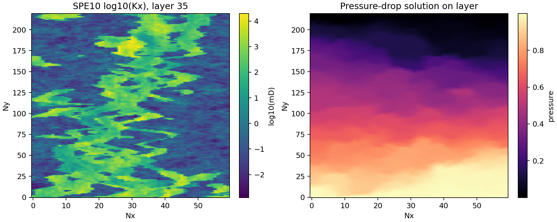
SPE10 case 2a layer visualization. Left: log10(Kx) on one physical layer. Right: pressure-drop solution on the same layer with unit pressure on the low-y side, zero pressure on the high-y side, and no-flow x/z boundaries.

Use --figure-mode 3d to generate a three-dimensional view of the full problem, or --figure-mode both to generate both figures:

examples/src/C_darcy/reproduce.sh --skip-run --figure-mode both

The figure generation lives in examples/src/C_darcy/postprocess.py and can also be run directly:

examples/src/C_darcy/postprocess.py \
   --result-file examples/src/C_darcy/reproduce-out/darcy_spe10.pvti \
   --mode both

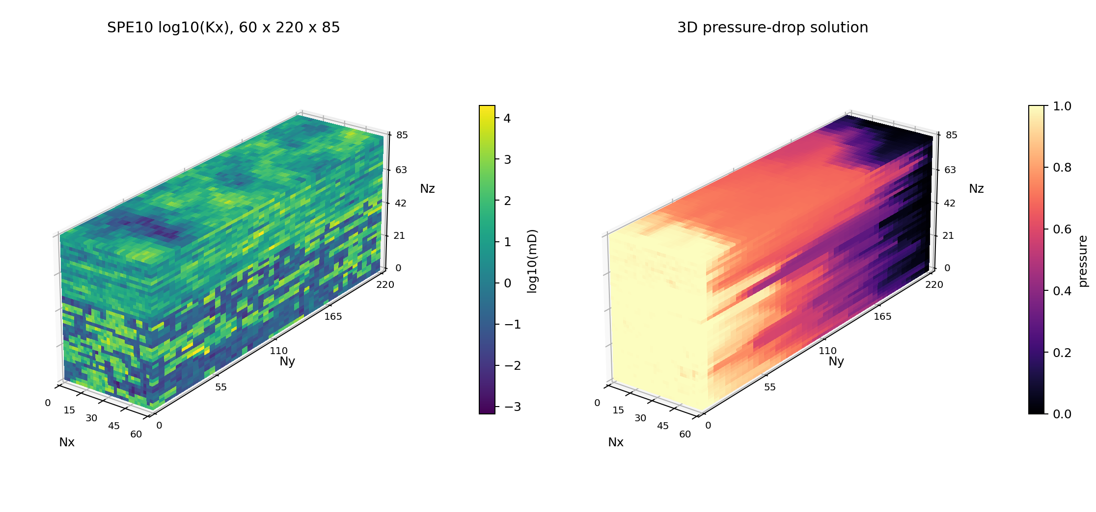
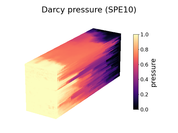
Full-volume SPE10 case 2a visualization using full-resolution exterior surfaces from the C Darcy VTK results. Left: log10(Kx) from the 60 x 220 x 85 permeability field. Right: pressure-drop solution on the same full-resolution grid, with unit pressure on the low-y side, zero pressure on the high-y side, and no-flow x/z boundaries.

The performance run uses the C mixed RT0/P0 driver:

mpirun -np 16 /path/to/build/darcy \
   -n 60 220 85 \
   -P 1 4 4 \
   --K-file data/spe10_case2a/spe_perm.dat \
   --K-file-grid 60 220 85 \
   --K-file-k-order top-down \
   --output examples/src/C_darcy/reproduce-out/darcy_spe10.vti \
   -g y -v 1

The figures are generated from the C VTK output with NumPy and Matplotlib, so reproducing the images does not require VTK or ParaView. Set SPE10_LAYER=<k> to choose a different physical layer for the layer figure. Set NP, NXYZ, PGRID, RESULT_FILE, BUILD_DIR, or DARCY_BIN to override the benchmark command. Use --skip-run or --skip-figure to run only one part.

MGR Preconditioning

The mixed operator is indefinite, so with HYPRE 3.x and newer the default configuration uses GMRES with a two-block MGR preconditioner. Flux rows are F-points and pressure rows are the coarse block:

solver:
  gmres:
    krylov_dim: 60
    max_iter: 200
    relative_tol: 1.0e-10
preconditioner:
  mgr:
    level:
      0:
        f_dofs: [1]
        f_relaxation: jacobi
        g_relaxation: none
        restriction_type: injection
        prolongation_type: jacobi
        coarse_level_type: rap
    coarsest_level:
      amg:
        max_iter: 1

This corresponds to eliminating/relaxing the flux block and applying BoomerAMG to the pressure Schur complement approximation. The C driver passes the dofmap with HYPREDRV_LinearSystemSetDofmap before attaching the IJ matrix and RHS, so MGR can identify the two fields.

With older HYPRE releases, the example uses a GMRES+BoomerAMG compatibility configuration because the MGR options exercised here require newer HYPRE APIs.

The driver also accepts hypredrive command-line overrides after -a or --args using the same path syntax as hypredrive-cli. Place these overrides after the Darcy-specific options:

mpirun -np 2 /path/to/build/darcy -n 30 110 85 -g x -v 1 \
   -a --solver:gmres:max_iter 100 --preconditioner:mgr:print_level 1

Preconditioner Strategy Comparison

Before comparing strategies, it helps to size the problem. On the full SPE10 grid the assembled system has 4,525,000 rows and 23,471,400 nonzeros, roughly 5.2 per row. It keeps the saddle-point block structure introduced above, with 3,403,000 flux rows and 1,122,000 pressure rows. The blocks are very different in density: the flux mass block \(M\) holds 10,071,200 nonzeros (about 2.96 per row, coupling each face to the same-direction faces of its neighbouring cells), the flux–pressure block \(B\) holds 6,668,200 (about 1.96 per flux row, one entry per cell a face borders), and \(B^{\top}\) holds 6,732,000 (exactly 6 per pressure row – the six faces of every cell). The pressure–pressure block is empty, so the operator is indefinite; this is exactly the structure the MGR splitting below is designed to exploit.

The flux/pressure splitting above leaves room for several preconditioner strategies. The example ships four MGR variants in examples/src/C_darcy/ that all converge on the SPE10 case but with different iteration counts:

• mgr_jacobi.yml – the default two-block MGR (Jacobi F-relaxation and a single BoomerAMG V-cycle on the pressure Schur complement).

• mgr_amg_strong.yml – strengthens the coarse (pressure) solve to two BoomerAMG V-cycles with l1-hybrid-SGS relaxation.

• mgr_ilu.yml – replaces the Jacobi flux relaxation with block-Jacobi ILU(0) (BJ-ILU0 F-relaxation).

• mgr_global_ilu.yml – keeps Jacobi F-relaxation but adds a global block-Jacobi ILU(0) smoother (BJ-ILU0 G-relaxation) over the full flux+pressure system.

Each strategy file sets print_level: 2 on the GMRES solver and statistics: 1, so every log carries both the per-iteration residual history and a setup/solve timing summary. A single loop captures one log per strategy on the SPE10 case:

cd examples/src/C_darcy
for s in mgr_jacobi mgr_amg_strong mgr_ilu mgr_global_ilu; do
  mpirun -np 16 /path/to/build/darcy -n 60 220 85 -P 1 4 4 \
     --K-file ../../../data/spe10_case2a/spe_perm.dat \
     --K-file-grid 60 220 85 --K-file-k-order top-down \
     -g y -v 1 -i ${s}.yml > ${s}.log
done

Two helper scripts turn those logs into a side-by-side comparison. scripts/plot_convergence.py (argparse-based; needs only the Python standard library and Matplotlib) parses the print_level: 2 history and plots the relative residual against the Krylov iteration, while scripts/analyze_statistics.py renders the setup/solve timing summary as a stacked bar chart (-m bar+setup+solve):

# Left panel: GMRES convergence history
../../../scripts/plot_convergence.py \
   mgr_amg_strong.log mgr_jacobi.log mgr_ilu.log mgr_global_ilu.log \
   --labels "MGR + strong coarse AMG" "MGR + Jacobi (default)" \
            "MGR + BJ-ILU0 F-relax" "MGR + BJ-ILU0 G-relax" \
   --title "SPE10 Darcy: GMRES convergence" -o convergence.png

# Right panel: stacked setup/solve time (HYPRE version read from the log)
cat mgr_amg_strong.log mgr_jacobi.log mgr_ilu.log mgr_global_ilu.log > combined.log
hv=$(grep -m1 HYPRE_RELEASE_VERSION combined.log | awk '{print $NF}')
../../../scripts/analyze_statistics.py -f combined.log -m bar+setup+solve \
   -ln "strong coarse AMG" "Jacobi (default)" "BJ-ILU0 F-relax" "BJ-ILU0 G-relax" \
   -T "SPE10 Darcy setup/solve time (HYPRE ${hv})" -s panel.png

# Place the two panels side by side
convert convergence.png stacked_bar_panel.png -resize x1100 +append \
   ../../../docs/usrman-src/figures/spe10_darcy_strategies.png

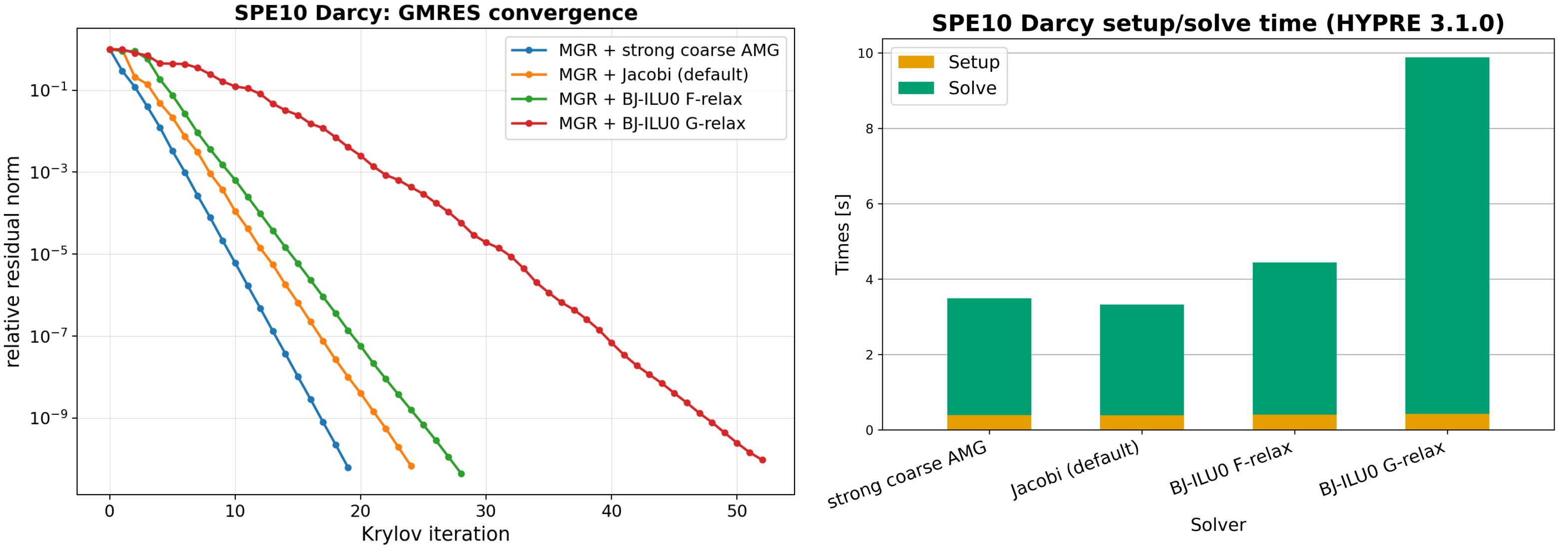
Left: GMRES relative residual versus Krylov iteration. Right: stacked setup/solve time per strategy. SPE10 case 2a Darcy problem (4.5M unknowns, 16 MPI ranks, relative_tol = 1e-10, HYPRE 3.1.0).

For this RT0/P0 system the flux mass block is well conditioned, so the cost is dominated by the quality of the pressure Schur-complement approximation. Strengthening the coarse pressure solve (mgr_amg_strong.yml) is the only change that lowers the iteration count, from 24 down to 19. Pouring more work into the flux block instead – BJ-ILU0 F-relaxation or a global BJ-ILU0 smoother – does not improve the Schur-complement approximation and only adds cost per iteration, so GMRES takes more iterations, not fewer.

The timing panel adds an important caveat: fewest iterations is not the same as fastest wall-clock. Each mgr_amg_strong iteration runs two l1-hybrid-SGS AMG cycles, so even though it needs the fewest iterations its solve time is slightly higher than the much cheaper default mgr_jacobi, which remains the best time-to-solution here. Setup time is small and nearly constant across strategies, so the solve phase dominates the total. For reference, a plain GMRES+BoomerAMG preconditioner without the MGR splitting stalls on the indefinite saddle-point system and fails to reach the tolerance within 200 iterations, which is why MGR is the default.

Reproducible Run

Build with examples enabled, then run:

mpirun -np 1 /path/to/build/darcy -n 4 3 1 -g x -v 1
mpirun -np 2 /path/to/build/darcy -n 4 3 1 -g x -v 1

The program prints the grid, unknown counts, MPI rank-grid and row-partition summary, drive direction, and relative cell-pressure L2 error against the analytic solution \(u=1-x_{\mathrm{axis}}/L_{\mathrm{axis}}\). The same executable accepts an external YAML file with -i to override the default GMRES+MGR options.

Example 3: Linear Elasticity

This section documents the mathematical model, discretization, and hypre usage for the 3D small-strain linear elasticity driver implemented in examples/src/C_elasticity/elasticity.c. It targets readers comfortable with PDEs, variational formulations, and finite element assembly.

Governing Equations (Small-Strain Isotropic Elasticity)

We consider a bounded Lipschitz domain \(\Omega \subset \mathbb{R}^3\) with boundary \(\partial\Omega = \Gamma_D \cup \Gamma_N\), \(\Gamma_D \cap \Gamma_N = \emptyset\). The unknown displacement field is \(\mathbf{u} : \Omega \to \mathbb{R}^3\).

• Kinematics (small strain):

  \[\varepsilon(\mathbf{u}) \;=\; \tfrac{1}{2}\big(\nabla \mathbf{u} + \nabla \mathbf{u}^\top\big) \;\in\; \mathbb{R}_{\text{sym}}^{3\times 3}.\]

• Constitutive law (isotropic Hooke):

  \[\sigma(\mathbf{u}) \;=\; \lambda\,\mathrm{tr}\!\big(\varepsilon(\mathbf{u})\big)\,I \;+\; 2G\,\varepsilon(\mathbf{u}),\]

  with Lamé parameters

  \[G \;=\; \frac{E}{2(1+\nu)},\qquad \lambda \;=\; \frac{E\nu}{(1+\nu)(1-2\nu)}.\]

• Strong form:

  \[-\nabla\!\cdot \sigma(\mathbf{u}) \;=\; \mathbf{f} \quad \text{in } \Omega, \qquad \mathbf{u} \;=\; \mathbf{0} \quad \text{on } \Gamma_D, \qquad \sigma(\mathbf{u})\,\mathbf{n} \;=\; \mathbf{t} \quad \text{on } \Gamma_N.\]

In the example driver: - The clamped plane is \(\Gamma_D = \{x=0\}\) (all three components fixed). - Body force \(\mathbf{f} = \rho\,\mathbf{g}\). - Optional traction \(\mathbf{t}\) on the top surface \(\{y=L_y\}\).

Variational Formulation

Let \(V = \big\{\mathbf{v}\in [H^1(\Omega)]^3 : \mathbf{v}=\mathbf{0}\text{ on }\Gamma_D\big\}\). The weak problem reads: find \(\mathbf{u} \in \mathbf{u}_D + V\) such that for all \(\mathbf{v} \in V\),

\[\int_{\Omega} \varepsilon(\mathbf{v}) : \sigma(\mathbf{u}) \, d\Omega \;=\; \int_{\Omega} \mathbf{v}\cdot \mathbf{f}\, d\Omega \;+\; \int_{\Gamma_N} \mathbf{v}\cdot \mathbf{t}\, d\Gamma.\]

With isotropy, in Voigt notation \(\varepsilon_v = (\varepsilon_{xx},\varepsilon_{yy},\varepsilon_{zz}, \gamma_{yz},\gamma_{xz},\gamma_{xy})^\top\), one writes \(\sigma_v = D\,\varepsilon_v\), where the \(6\times6\) matrix \(D\) is

\[\begin{split}D \;=\; \begin{bmatrix} \lambda+2G & \lambda & \lambda & 0 & 0 & 0 \\ \lambda & \lambda+2G & \lambda & 0 & 0 & 0 \\ \lambda & \lambda & \lambda+2G & 0 & 0 & 0 \\ 0 & 0 & 0 & G & 0 & 0 \\ 0 & 0 & 0 & 0 & G & 0 \\ 0 & 0 & 0 & 0 & 0 & G \end{bmatrix}.\end{split}\]

Discretization: Q1 Hexahedra on a Cartesian Mesh

We use a uniform Cartesian mesh with nodal counts \(N=(N_x,N_y,N_z)\) and physical sizes \(L=(L_x,L_y,L_z)\). Element sizes are \(h = (h_x,h_y,h_z) = \big(L_x/(N_x-1),\, L_y/(N_y-1),\, L_z/(N_z-1)\big)\). Each hexahedral element has 8 vertices with trilinear (Q1) shape functions on the reference cube \(\widehat{\Omega}=[-1,1]^3\).

Reference shape functions and derivatives

Number the element vertices \(a=1,\dots,8\) and define signed tuples \((s_x^a,s_y^a,s_z^a)\in\{\pm1\}^3\). The reference shape functions are

\[N_a(\xi,\eta,\zeta) \;=\; \tfrac{1}{8}\,(1+s_x^a \xi)\,(1+s_y^a \eta)\,(1+s_z^a \zeta),\]

with derivatives

\[\begin{split}\frac{\partial N_a}{\partial \xi} \;=\; \tfrac{1}{8}\,s_x^a\,(1+s_y^a \eta)\,(1+s_z^a \zeta),\\ \frac{\partial N_a}{\partial \eta} \;=\; \tfrac{1}{8}\,s_y^a\,(1+s_x^a \xi)\,(1+s_z^a \zeta),\\ \frac{\partial N_a}{\partial \zeta} \;=\; \tfrac{1}{8}\,s_z^a\,(1+s_x^a \xi)\,(1+s_y^a \eta).\end{split}\]

Mapping and gradient transformation

For a uniform rectangular element the mapping \(\mathbf{x}(\xi,\eta,\zeta)\) has constant Jacobian

\[J \;=\; \mathrm{diag}\!\big(\tfrac{h_x}{2},\,\tfrac{h_y}{2},\,\tfrac{h_z}{2}\big),\qquad J^{-1} \;=\; \mathrm{diag}\!\big(\tfrac{2}{h_x},\,\tfrac{2}{h_y},\,\tfrac{2}{h_z}\big),\qquad \det J \;=\; \tfrac{h_x h_y h_z}{8}.\]

Physical gradients follow from \(\nabla_{\mathbf{x}} N_a = J^{-\top}\,\nabla_{\xi} N_a\), i.e.,

\[\frac{\partial N_a}{\partial x} \;=\; \frac{2}{h_x}\,\frac{\partial N_a}{\partial \xi},\qquad \frac{\partial N_a}{\partial y} \;=\; \frac{2}{h_y}\,\frac{\partial N_a}{\partial \eta},\qquad \frac{\partial N_a}{\partial z} \;=\; \frac{2}{h_z}\,\frac{\partial N_a}{\partial \zeta}.\]

Strain–displacement operator (Voigt form)

Let \(\mathbf{u}_e \in \mathbb{R}^{24}\) collect the 24 element dofs in the interleaved order \([u_{x1},u_{y1},u_{z1},\,\dots,\,u_{x8},u_{y8},u_{z8}]^\top\). The strain in Voigt notation \(\varepsilon_v = (\varepsilon_{xx},\varepsilon_{yy},\varepsilon_{zz}, \gamma_{yz},\gamma_{xz},\gamma_{xy})^\top\) is

\[\varepsilon_v(\mathbf{u}_e) \;=\; B\,\mathbf{u}_e,\qquad B \;=\; \big[\,B_1\;\;B_2\;\;\cdots\;\;B_8\,\big],\;\; B_a \in \mathbb{R}^{6\times 3},\]

with per-node blocks

\[\begin{split}B_a \;=\; \begin{bmatrix} \partial_x N_a & 0 & 0 \\ 0 & \partial_y N_a & 0 \\ 0 & 0 & \partial_z N_a \\ 0 & \partial_z N_a & \partial_y N_a \\ \partial_z N_a & 0 & \partial_x N_a \\ \partial_y N_a & \partial_x N_a & 0 \end{bmatrix}.\end{split}\]

Element matrices and loads

• Volume quadrature: tensor-product 2×2×2 Gauss points \(\{(\xi_q,\eta_q,\zeta_q),\,w_q\}\). With the constant mapping, the physical weight is \(w_q^{\Omega} = w_q \,\det J\). The element stiffness and body-force load read

  \[K_e \;=\; \sum_q B(\xi_q,\eta_q,\zeta_q)^\top\, D \, B(\xi_q,\eta_q,\zeta_q)\; w_q^{\Omega}, \qquad \mathbf{f}_e^{\text{vol}} \;=\; \sum_q N(\xi_q,\eta_q,\zeta_q)^\top (\rho\,\mathbf{g})\; w_q^{\Omega},\]

  where \(N(\cdot)\in\mathbb{R}^{3\times 24}\) is the vector-valued shape function matrix that places each scalar \(N_a\) on the three displacement components in the interleaved ordering.

• Traction on the top face \(\{y=L_y\}\) corresponds to \(\eta = +1\) on the reference element. Using 2×2 Gauss in \((\xi,\zeta)\) with surface Jacobian \(\det J_s=\tfrac{h_x h_z}{4}\), the face load contribution is

  \[\mathbf{f}_e^{\text{trac}} \;=\; \sum_{q\in \widehat{\Gamma}} N(\xi_q,\,\eta{=}+1,\,\zeta_q)^\top \,\mathbf{t}\; w_q^{\Gamma},\qquad w_q^{\Gamma} \;=\; w_q \,\det J_s.\]

In practice, the driver precomputes the constant factors (e.g., \(J^{-1}\), \(\det J\), and the values of \(B\) at Gauss points) to amortize cost across elements with identical size, and assembles \(K_e\) and \(\mathbf{f}_e=\mathbf{f}_e^{\text{vol}}+\mathbf{f}_e^{\text{trac}}\) into the global system using the interleaved dof map.

Element Matrices and Vectors

For a single element with 8 nodes and 3 components per node (24 dofs), define the element strain-displacement operator \(B(\xi,\eta,\zeta) \in \mathbb{R}^{6\times 24}\) in Voigt form, assembled from the physical derivatives \((\partial N_a/\partial x,\partial N_a/\partial y,\partial N_a/\partial z)\). The element stiffness and loads are

\[K_e \;=\; \int_{\Omega_e} B^\top D\,B\, d\Omega \;\;\approx\;\; \sum_{q\in Q_{2\times2\times2}} B_q^\top D\,B_q\, w_q,\]

\[\mathbf{f}_e^{\text{vol}} \;=\; \int_{\Omega_e} N^\top\,(\rho\,\mathbf{g})\, d\Omega \;\;\approx\;\; \sum_{q\in Q_{2\times2\times2}} N_q^\top\,(\rho\,\mathbf{g})\, w_q,\]

\[\mathbf{f}_e^{\text{trac}} \;=\; \int_{\Gamma_{t}\cap\partial\Omega_e} N^\top\,\mathbf{t}\, d\Gamma \;\;\approx\;\; \sum_{q\in Q_{2\times2}} N_q^\top\,\mathbf{t}\, w_q^{\Gamma}.\]

Boundary Conditions and SPD Structure

The clamped plane \(\{x=0\}\) imposes \(\mathbf{u}=\mathbf{0}\) on all three displacement components. In assembly, we:

1. Suppress all rows and columns associated with Dirichlet dofs when inserting element contributions.

2. Before final assembly, set each Dirichlet row to an identity row (diagonal 1) and RHS 0.

This yields a symmetric positive definite (SPD) system.

Parallel Partitioning and Global Numbering

We use an MPI Cartesian partition \(P=(P_x,P_y,P_z)\). Let \(pstarts[d][b]\) be the prefix-sum array of node starts along dimension \(d\) for block coordinate \(b\in\{0,\dots,P_d\}\) (balanced remainder). Denote the owner of global node \((i,j,k)\) by \((b_x,b_y,b_z)\). The scalar global node ID uses lexicographic ordering with block-aware offsets (as in grid2idx). With three interleaved displacement components per node, DOF IDs satisfy:

\[\mathrm{dof}_{\mathrm{gid}}(a,c) \;=\; 3\,\mathrm{node}_{\mathrm{gid}}(a) \;+\; c, \qquad c\in\{0,1,2\}.\]

The driver restricts insertion to owned rows; off-rank columns (couplings) are allowed by IJ assembly.

Linear System Creation

• Create HYPRE_IJMatrix and HYPRE_IJVector on the solver communicator with global dof bounds for this rank; set object type to HYPRE_PARCSR.

• Provide per-row nnz upper bounds (conservative 81) with HYPRE_IJMatrixSetRowSizes; initialize with HYPRE_IJMatrixInitialize_v2 and HYPRE_IJVectorInitialize_v2.

• Assemble element contributions using HYPRE_IJMatrixAddToValues and HYPRE_IJVectorAddToValues.

• Impose Dirichlet rows with HYPRE_IJMatrixSetValues and HYPRE_IJVectorSetValues.

• Finalize with HYPRE_IJMatrixAssemble and HYPRE_IJVectorAssemble.

• Optional GPU migration with HYPRE_IJMatrixMigrate/HYPRE_IJVectorMigrate if built with GPU.

For example, the following code snippet shows how to create a HYPRE_IJMatrix and HYPRE_IJVector and assemble element contributions using HYPRE_IJMatrixAddToValues and HYPRE_IJVectorAddToValues and set the linear system components to hypredrive. Note that the interleaved 3-DOF layout per node is announced to hypredrive before setting the matrix and vector components. This information might be useful for some preconditioners.

HYPRE_IJMatrix A;
HYPRE_IJVector b;
/* ... create/initialize/insert/assemble A, b ... */

HYPREDRV_LinearSystemSetInterleavedDofmap(hdrv, local_num_nodes, 3);
HYPREDRV_LinearSystemSetMatrix(hdrv, (HYPRE_Matrix)A);
HYPREDRV_LinearSystemSetRHS(hdrv, (HYPRE_Vector)b);
HYPREDRV_LinearSystemSetInitialGuess(hdrv, NULL);
HYPREDRV_LinearSystemSetPrecMatrix(hdrv, NULL);

Near-Nullspace and Rigid Body Modes (RBMs)

For linear elasticity, the near-nullspace of the operator (particularly under weak constraints) is spanned by the six rigid body modes (RBMs):

• three translations: \(t_x=(1,0,0)\), \(t_y=(0,1,0)\), \(t_z=(0,0,1)\)

• three rotations about the domain center \(\mathbf{c}=(L_x/2, L_y/2, L_z/2)\): \(\mathbf{u}(\mathbf{x})=\boldsymbol{\omega}\times(\mathbf{x}-\mathbf{c})\) with \(\boldsymbol{\omega}\in\{(1,0,0),(0,1,0),(0,0,1)\}\)

Supplying RBMs to the preconditioner (e.g., BoomerAMG) may improve robustness and convergence, especially when using nodal coarsening for vector-valued problems. From the HYPREDRV perspective:

• The elasticity driver computes the six RBMs on the physical mesh coordinates.

• The modes are arranged in component-major (SoA) order: six contiguous blocks, each of length num_entries = 3 * num_local_nodes (interleaved dofs per node).

• Dirichlet-clamped DOFs (the plane x=0 in this example) are explicitly zeroed in all modes.

• The application transfers the modes to hypre with a single call; the data is copied internally by libHYPREDRV, so the application can free its buffer afterwards.

Driver-side mode computation

In the example driver, a helper computes the six RBMs using physical coordinates scaled by the input dimensions \(L=(L_x, L_y, L_z)\) and zeros clamped DOFs:

/* Compute 6 modes (Tx, Ty, Tz, Rx, Ry, Rz) into a single contiguous array.
   Each block has length num_entries = 3 * local_num_nodes (interleaved dofs per node). */
extern int ComputeRigidBodyModes(DistMesh *mesh, ElasticParams *params, HYPRE_Real **rbm_ptr);

/* ... after BuildElasticitySystem_Q1Hex(...) */
HYPRE_Real *rbm = NULL;
const int num_entries   = 3 * mesh->local_size;
const int num_components = 6;
ComputeRigidBodyModes(mesh, &params, &rbm);
/* rbm layout (SoA): [Tx block | Ty block | Tz block | Rx block | Ry block | Rz block] */

/* Tell libHYPREDRV about the near-nullspace modes (data is copied internally; free rbm afterwards) */
HYPREDRV_LinearSystemSetNearNullSpace(hdrv, num_entries, num_components, rbm);
free(rbm);

Using RBMs in libHYPREDRV

• Provide the six-mode buffer as above before creating the preconditioner and solver.

• Hypredrive stores the near-nullspace vector internally and can pass it to the configured preconditioner. For BoomerAMG nodal coarsening, typical settings involve:

  preconditioner:
    amg:
      coarsening:
        nodal: 1   # Nodal coarsening based on row-sum norm (default)
      # optional advanced controls (implementation-dependent):
      # interpolation:
      #   ...
      # relaxation:
      #   ...
  

• Memory and layout: - The call HYPREDRV_LinearSystemSetNearNullSpace(h, num_entries, num_components, values) expects the values in SoA layout: num_components contiguous blocks, each with num_entries degrees of freedom. - The buffer is copied into libHYPREDRV-owned storage; the caller must free its buffer after the call returns.

Note

Near null space modes are distinct from the exact null space modes set with HYPREDRV_LinearSystemSetNullSpace(): near null space modes inform the preconditioner construction and are not projected out of the solution, while exact null space modes are projected out of every computed solution to fix its gauge (see the Q2-Q1 lid-driven cavity discretization below). The rigid body modes of a clamped elastic body, as in this example, are near null space modes but not exact ones.

Linear Solver Setup

The linear solver is created, setup, applied, and destroyed per solve. Solver and preconditioner choices (e.g., PCG/FGMRES, AMG/MGR), tolerances, stopping criteria, and other options are provided via the YAML configuration parsed earlier with HYPREDRV_InputArgsParse; the create/setup/apply sequence below honors those settings.

HYPREDRV_LinearSolverCreate(hdrv);
HYPREDRV_LinearSolverSetup(hdrv);
HYPREDRV_LinearSolverApply(hdrv);
HYPREDRV_LinearSolverDestroy(hdrv);

The default in the example is a conjugate gradient solver with an unknown-based BoomerAMG preconditioner (Prolongation operator considers only intra-variable couplings, i.e., connections within the same type of displacement component).

Solver Comparison

The elasticity driver now exposes a dedicated --solver-preset option to exercise both built-in and application-registered preconditioner presets from the command line. The available values are:

• elasticity_3D: built-in BoomerAMG elasticity preset.

• elasticity_sdc_3D: application-registered preset that matches elasticity_3D and additionally sets coarsening.filter_functions: on.

• elasticity_nodal_3D: application-registered preset that matches elasticity_3D and additionally sets coarsening.nodal: 1.

The two custom presets are registered at runtime by the application via HYPREDRV_PreconPresetRegister before parsing YAML or applying command-line overrides. They are therefore example-local conveniences and not global built-in presets.

To compare all three configurations over a DOF sweep (8 variants from about 1e4 to 1e6 unknowns), run:

./reproduce.sh

The script runs each preset across all size variants, stores outputs in elasticity_builtin.out, elasticity_sdc.out, and elasticity_nodal.out, and then always generates plots by default. It calls scripts/analyze_statistics.py with -t rows and --log-x to produce separate comparison figures with a log-scale X axis (DOFs):

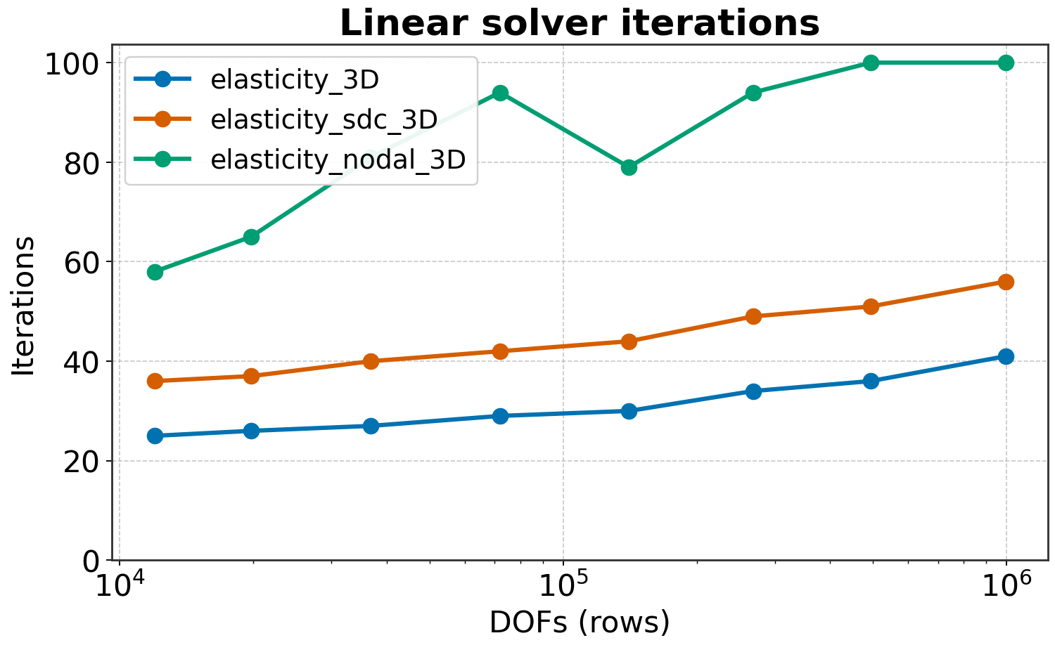
Linear solver iterations vs DOFs.

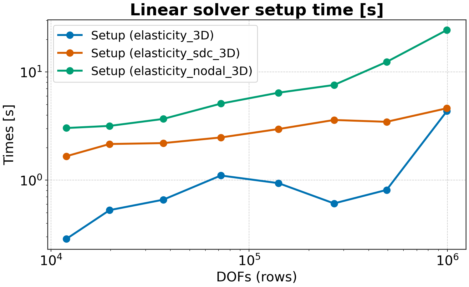
Preconditioner setup time vs DOFs.

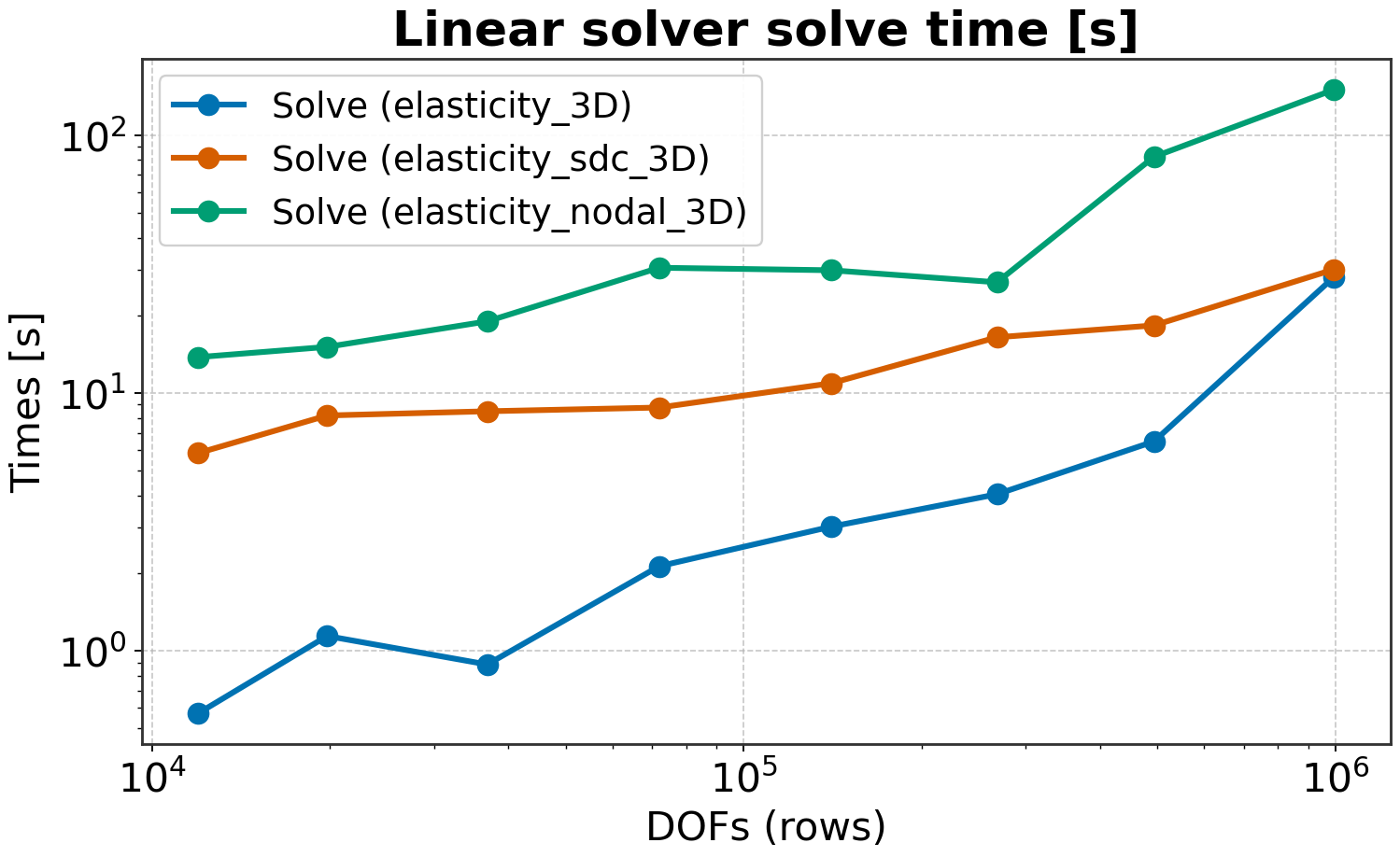
Solve time vs DOFs.

The script prints verbose messages indicating which plot is being generated.

To regenerate only the plots from existing *.out logs (without rerunning solves):

./reproduce.sh --plot-only

Visualizing the Solution

The driver can emit per-rank VTK RectilinearGrid pieces with one-layer overlap on the negative faces so adjacent subdomains stitch seamlessly. Ghost data for faces, edges, and corners are exchanged prior to writing to avoid cracks at partition boundaries.

• -vis 1: ASCII VTK. Easy to inspect/diff but larger on disk and slower to write.

• -vis 2: Appended raw binary. Compact and faster; preferred for larger runs.

Output artifacts:

• One file per rank: elasticity_{Nx}x{Ny}x{Nz}_{Px}x{Py}x{Pz}_{rank}.vtr with a 3-component point vector named displacement.

• One collection file on rank 0: elasticity_{Nx}x{Ny}x{Nz}_{Px}x{Py}x{Pz}.pvd enumerating all rank pieces.

To visualize, open the .pvd in ParaView. Display the displacement vector and, optionally, use “Warp By Vector” or “Glyph” filters to view deformations or vectors.

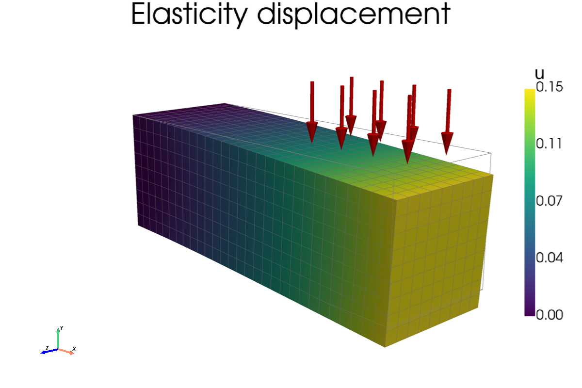
Displacement field rendered with PyVista. The deformed (warped) configuration is colored by magnitude \(\|\mathbf{u}\|_2 = \sqrt{u_x^2 + u_y^2 + u_z^2}\) (modest warp scale) and shown together with the original (undeformed) configuration as a light box outline. The red arrows on the free-end top surface mark the downward load that bends the cantilever.

The bundled postprocess.py (PyVista) generates this from the -vis output:

mpirun -np 4 /path/to/build/elasticity -P 2 2 1 -vis 2
python3 postprocess.py elasticity_30x10x10_2x2x1.pvd -o elasticity_solution_3d.png   # needs: pip install pyvista

Reproducible Run

Command-line parameters (see elasticity -h) control problem size, partitioning, material/loads, verbosity, and visualization. Defaults (in parentheses) match the figure above and the reference output included below.

mpirun -np 1 /path/to/build/examples/src/C_elasticity/elasticity -h

Usage: ${MPIRUN} ./elasticity [options]

Options:
  -i <file>         : YAML configuration file for solver settings (Optional)
  -n <nx> <ny> <nz> : Global grid dimensions in nodes (30 10 10)
  -P <Px> <Py> <Pz> : Processor grid dimensions (1 1 1)
  -L <Lx> <Ly> <Lz> : Physical dimensions (3 1 1)
  -g <gx> <gy> <gz> : Gravity vector g (0 -9.81 0)
  -T <tx> <ty> <tz> : Uniform traction on top surface y=Ly (0 -100 0)
  -br <n>           : Batch rows for matrix assembly (128)
  -E <val>          : Young's modulus E (1.0e5)
  -nu <val>         : Poisson ratio nu (0.3)
  -rho <val>        : Density rho (1.0)
  --solver-preset <name>
                   : Solver preset selector (elasticity_3D | elasticity_sdc_3D | elasticity_nodal_3D)
  -ns|--nsolve <n>  : Number of solves (5)
  -vis <m>          : Visualization mode (0)
      0: none
      1: ASCII VTK
      2: binary VTK
  -v|--verbose <n>  : Verbosity bitset (0)
      0x1: Library info and linear solver statistics
      0x2: System info
      0x4: Print linear system matrices
  -h|--help         : Print this message

For a single-process run, the output should be similar to the following:

mpirun -np 1 /path/to/build/examples/src/C_elasticity/elasticity

Date and time: YYYY-MM-DD HH:MM:SS

Using HYPREDRV_DEVELOP_STRING: HYPREDRV_VERSION_GOES_HERE

Running on 1 MPI rank

=====================================================
          Linear Elasticity Problem Setup
=====================================================
Physical dimensions:     3 x 1 x 1
Grid dimensions (nodes): 30 x 10 x 10
Processor topology:      1 x 1 x 1
Material:                E=1.0e+05, nu=0.300
Body force:              rho=1.0e+00, g=(0.0, -9.8, 0.0)
Top traction:            t=(0.0e+00, -1.0e+02, 0.0e+00)
Visualization:           false
Verbosity level:         0x3
Number of solves:        5
=====================================================

Assembling linear system... Done!
Solve 1/5...
Solve 2/5...
Solve 3/5...
Solve 4/5...
Solve 5/5...
====================================================================================


STATISTICS SUMMARY:

+--------+-------------+-------------+-------------+------------+------------+--------+
|        |    LS build |       setup |       solve |    initial |   relative |        |
|  Entry |   times [s] |   times [s] |   times [s] |  res. norm |  res. norm |  iters |
+--------+-------------+-------------+-------------+------------+------------+--------+
|      0 |       0.018 |       0.017 |       0.041 |   1.79e+01 |   2.66e-07 |     21 |
|      1 |             |       0.016 |       0.043 |   1.79e+01 |   2.66e-07 |     21 |
|      2 |             |       0.017 |       0.044 |   1.79e+01 |   2.66e-07 |     21 |
|      3 |             |       0.017 |       0.043 |   1.79e+01 |   2.66e-07 |     21 |
|      4 |             |       0.016 |       0.042 |   1.79e+01 |   2.66e-07 |     21 |
+--------+-------------+-------------+-------------+------------+------------+--------+

Date and time: YYYY-MM-DD HH:MM:SS
/home/victor/projects/hypredrive-master/build-v3.0.0/elasticity done!

Example 4: Nonlinear Heat Flow

This section documents the transient nonlinear heat conduction driver implemented in examples/src/C_heatflow/heatflow.c. It solves a scalar diffusion equation with temperature-dependent conductivity on a structured 3D mesh using Q1 hexahedral elements, backward Euler time integration, and a full Newton method.

Geometry and Boundary Conditions

The domain is \(\Omega = [0, L_x] \times [0, L_y] \times [0, L_z]\) with a Cartesian grid of \(N_x \times N_y \times N_z\) nodes. The y-axis represents the vertical direction with a cold base:

• Dirichlet: \(T = 0\) on the bottom plane \(y = 0\) (cold base)

• Neumann (insulated): \(\partial T / \partial n = 0\) on all other faces (\(x = 0\), \(x = L_x\), \(y = L_y\), \(z = 0\), \(z = L_z\))

This configuration models heat conduction in a body with an isothermal cold base and thermally insulated sides and top.

Governing Equation

We consider the PDE

\[\rho c\, \partial_t T \;-\; \nabla\!\cdot\!\big(k(T)\,\nabla T\big) \;=\; Q_{\text{MMS}}(x,y,z,t), \qquad k(T) \;=\; k_0\,e^{\beta T}.\]

The nonlinear conductivity \(k(T)\) allows modeling temperature-dependent thermal properties:

• \(\beta = 0\): linear conductivity (\(k = k_0\))

• \(\beta > 0\): conductivity increases with temperature

• \(\beta < 0\): conductivity decreases with temperature

MMS Validation

The example uses a transient Method of Manufactured Solutions (MMS) with a 3D exact solution:

\[T_{\text{exact}}(x,y,z,t) \;=\; e^{-t}\, \frac{1 + \cos(2\pi x/L_x)}{2}\, \sin\!\left(\frac{\pi y}{2 L_y}\right)\, \frac{1 + \cos(2\pi z/L_z)}{2},\]

which satisfy the boundary conditions:

• \(T = 0\) at \(y = 0\) (since \(\sin(0) = 0\))

• \(\partial T / \partial x = 0\) at \(x = 0, L_x\) (since \(\sin(0) = \sin(2\pi) = 0\))

• \(\partial T / \partial y = 0\) at \(y = L_y\) (since \(\cos(\pi/2) = 0\))

• \(\partial T / \partial z = 0\) at \(z = 0, L_z\) (since \(\sin(0) = \sin(2\pi) = 0\))

The corresponding source term \(Q_{\text{MMS}}\) is computed analytically so that \(T_{\text{exact}}\) satisfies the PDE, enabling verification of the numerical implementation. The solution has full 3D spatial variation, with temperature maxima at the corners \((0,L_y,0)\) and \((L_x,L_y,L_z)\) and minima along the \(y=0\) plane.

Discretization and Nonlinear Formulation

• Space: trilinear Q1 hexahedral elements on a uniform Cartesian grid.

• Time: backward Euler (implicit, first order).

• Unknown: scalar temperature, one DOF per node.

• Nonlinear conductivity: \(k(T)=k_0 e^{\beta T}\), so \(k'(T)=\beta k(T)\).

At a Newton iterate \(T^k\) the residual reads

\[R(T^k) \;=\; \frac{\rho c}{\Delta t}\,M\,(T^k - T^n) \;+\; \int_{\Omega} k(T^k)\,\nabla v \cdot \nabla T^k \, d\Omega \;-\; \int_{\Omega} v\,Q_{\text{MMS}} \, d\Omega.\]

The Jacobian applied to \(\delta T\) is

\[J(T^k)\,\delta T \;=\; \frac{\rho c}{\Delta t}\,M\,\delta T \;+\; \int_{\Omega} k(T^k)\,\nabla v \cdot \nabla(\delta T) \, d\Omega \;+\; \int_{\Omega} k'(T^k)\,(\delta T)\,\big(\nabla v \cdot \nabla T^k\big) \, d\Omega.\]

Implementation notes:

• Precomputed Q1 templates provide consistent mass and unit-diffusion stiffness on uniform hexes; conductivity and nonlinear terms are accumulated at Gauss points.

• Dirichlet rows are set to identity with zero RHS (Newton solves for the update), and interior rows include zero entries for Dirichlet columns to preserve a symmetric sparsity pattern (AMG friendly).

• Parallel assembly uses face/edge/corner ghost exchanges so each rank can evaluate boundary-straddling elements without cracks in the global solution or VTK output.

Jacobian Symmetry and Solver Choice

The Jacobian matrix is symmetric only when \(\beta = 0\) (linear conductivity). For nonlinear conductivity (\(\beta \neq 0\)), the extra Jacobian term

\[\int_{\Omega} k'(T^k)\,(\delta T)\,\big(\nabla v \cdot \nabla T^k\big)\, d\Omega\]

introduces asymmetry because \(\nabla v \cdot \nabla T^k\) differs from \(\nabla(\delta T) \cdot \nabla T^k\) when expanded in the finite element basis.

• PCG (conjugate gradient) works correctly for \(\beta = 0\) and may work for small \(|\beta|\) where the asymmetry is negligible.

• GMRES (or FGMRES) is recommended for nonlinear problems (\(\beta \neq 0\)) as it handles non-symmetric systems robustly. The default configuration uses GMRES+AMG for this reason.

Output and Diagnostics

• VTK RectilinearGrid per rank with point fields:

  • temperature (numerical solution)

  • conductivity (derived via \(k(T)\))

  • temperature_exact (MMS exact solution, enable with -vis 16 bit)

  • heat_flux vector field \(\mathbf{q}=-k(T)\nabla T\) (enable with -vis 8 bit)

• PVD collection at the end for easy time series loading in ParaView.

• The header and iteration logs report:

  • Fourier number \(\text{Fo} = \alpha_0 \Delta t / h_{\min}^2\) where \(\alpha_0 = k_0 / (\rho c)\)

  • Total internal energy \(E = \int_\Omega \rho c\, T\, d\Omega\) and \(\Delta E\) per step

  • MMS L2 error \(\|T - T_{\text{exact}}\|_{L^2}\) at each Newton iteration

Reproducible Run

Usage: mpirun -np <np> ./heatflow [options]

Options:
  -i <file>         : YAML configuration file for solver settings
  -n <nx> <ny> <nz> : Global grid nodes (default: 17 17 17)
  -P <Px> <Py> <Pz> : Processor grid (default: 1 1 1)
  -L <Lx> <Ly> <Lz> : Domain lengths (default: 1 1 1)
  -rho <val>        : Density (default: 1)
  -cp <val>         : Heat capacity (default: 1)
  -dt <val>         : Time step (default: 1e-2)
  -tf <val>         : Final time (default: 1.0)
  -k0 <val>         : Base conductivity (default: 1)
  -beta <val>       : Conductivity exponent (default: 0 = linear)
  -br <n>           : Batch rows per IJ call (default: 128)
  -adt              : Enable adaptive time stepping
  -cfl <val>        : Maximum CFL for adaptive time stepping (0=no limit)
  -vis <m>          : Visualization mode bitset (default: 0)
                       Any nonzero value enables visualization
                       Bit 1 (0x2): ASCII (1) or binary (0)
                       Bit 2 (0x4): All timesteps (1) or last only (0)
                       Bit 3 (0x8): Include heat flux in output
                       Bit 4 (0x10): Include exact MMS solution
  -nw_max <n>       : Newton max iterations (default: 20)
  -nw_tol <t>       : Newton update tolerance ||delta||_inf (default: 1e-5)
  -nw_rtol <t>      : Newton residual tolerance ||R||_2 (default: 1e-5)
  -v|--verbose <n>  : Verbosity bitset (default: 7)
                       0x1: Newton iteration info
                       0x2: Library and system info
                       0x4: Print linear system
  -h|--help         : Print this message

# 2×2×2 parallel, transient MMS with insulated BCs, moderate nonlinearity
mpirun -np 8 ./heatflow -n 33 33 33 -P 2 2 2 -beta 0.5 -dt 0.01 -tf 0.1 -v 1

Transient Visualization

Enabling all-timestep VTK output (-vis 4) writes a .pvd time-series collection that the bundled postprocess.py renders into an animated GIF of the temperature isosurfaces with PyVista. The -cfl 1.0 flag caps the time-step size so the frames are uniformly spaced across the transient (otherwise the driver grows dt and only a handful of frames are produced).

mpirun -np 4 /path/to/build/heatflow -n 49 49 49 -P 2 2 1 -dt 0.005 -tf 0.6 -cfl 1.0 -vis 4
python3 postprocess.py heatflow_49x49x49_2x2x1.pvd -o heatflow_transient.gif   # needs: pip install pyvista imageio

Nested translucent isosurfaces of the temperature field over the transient. The hot cores at the insulated corners gradually shrink and cool as heat diffuses out through the isothermal cold base at \(y = 0\); the isosurface levels and color scale are held fixed so the decay is apparent.

Example 5: Lid-Driven Cavity (Navier-Stokes)

This section documents the mathematical model, discretization, and hypre usage for the 2D lid-driven cavity driver implemented in examples/src/C_lidcavity/lidcavity.c. This is a classical benchmark problem for incompressible fluid flow solvers, featuring time-dependent Navier-Stokes equations solved with stabilized finite elements and Newton iteration.

Governing Equations (Incompressible Navier-Stokes)

We consider the unit square domain \(\Omega = [0, L] \times [0, L]\) with the lid-driven cavity configuration. The unknowns are the velocity field \(\mathbf{u} = (u, v)\) and the pressure \(p\).

• Momentum equation:

  \[\frac{\partial \mathbf{u}}{\partial t} + (\mathbf{u} \cdot \nabla) \mathbf{u} - \nu \nabla^2 \mathbf{u} + \nabla p = \mathbf{0} \quad \text{in } \Omega,\]

• Continuity equation (incompressibility):

  \[\nabla \cdot \mathbf{u} = 0 \quad \text{in } \Omega,\]

where the kinematic viscosity \(\nu = 1/\text{Re}\) is the inverse of the Reynolds number.

Geometry and Boundary Conditions

The lid-driven cavity is a square domain with the following boundary conditions:

• Lid (\(y = L\), excluding corners): \(u = u_{\text{lid}}(x)\), \(v = 0\)

  • Classic BC: \(u_{\text{lid}} = 1\) (discontinuous at corners)

  • Regularized BC: \(u_{\text{lid}} = [1 - (2x/L - 1)^{16}]^2\) (smooth, zero at corners)

• Walls (\(x = 0\), \(x = L\), \(y = 0\), and corners): \(\mathbf{u} = \mathbf{0}\) (no-slip)

• Pressure: Fixed at one node (bottom-left corner, \(p = 0\)) to remove the nullspace

The regularized boundary condition eliminates the velocity discontinuity at the top corners, which can cause numerical difficulties at high Reynolds numbers.

Numerical Discretization

This section describes the spatial and temporal discretization of the lid-driven cavity problem.

Spatial Discretization

By default, we use equal-order bilinear (Q1) finite elements for both velocity and pressure on a structured quadrilateral mesh. This violates the Ladyzhenskaya-Babuška-Brezzi (LBB) inf-sup condition, requiring stabilization to obtain a well-posed system. In this discretization, the three degrees of freedom (u, v, p) are interleaved at every node and the pressure is pinned at a reference node.

Alternatively, the driver supports an inf-sup stable Q2-Q1 (Taylor-Hood) discretization via the -disc q2q1 command line option, which requires no stabilization. The -n option then gives the pressure (bilinear) grid, while the velocity (biquadratic) grid has (2*nx - 1) x (2*ny - 1) nodes. Because the two fields live on staggered grids with different numbers of unknowns, the degrees of freedom are stored in a block layout — (u, v) pairs interleaved over the velocity nodes followed by the pressure block — and the dof types are communicated to hypredrive with explicit labels (HYPREDRV_LinearSystemSetDofmap() with u = 0, v = 1, p = 2) instead of the interleaved dofmap helper. Moreover, the pressure is not pinned in this mode: since the enclosed flow determines the pressure only up to a constant, the example registers the constant pressure mode with HYPREDRV_LinearSystemSetNullSpace() and hypredrive projects it out of the solution after every solve, fixing the pressure gauge. The default solver configuration for -disc q2q1 is a two-level MGR preconditioner with the velocity dof types as F points, the pressure as the C point, and blk-absrowsum prolongation. The Q2-Q1 path runs in serial and in parallel (-P Px Py); hypre requires at least version 3.1 for the MGR default configuration.

The two discretizations can be compared side by side with examples/src/C_lidcavity/compare.sh, which sweeps Reynolds and CFL numbers at matched velocity resolution and reports time steps, nonlinear/linear iteration counts, the final kinetic energy (a solution observable printed by the driver and comparable between the discretizations), and wall times.

Temporal Discretization

Backward Euler (implicit, first-order) is used for time integration:

\[\frac{\mathbf{u}^{n+1} - \mathbf{u}^n}{\Delta t} + (\mathbf{u}^{n+1} \cdot \nabla) \mathbf{u}^{n+1} - \nu \nabla^2 \mathbf{u}^{n+1} + \nabla p^{n+1} = \mathbf{0}\]

The nonlinear convective term is handled by Newton iteration within each time step.

SUPG and PSPG Stabilization

To stabilize the equal-order discretization, we add SUPG (Streamline-Upwind/Petrov-Galerkin) for the momentum equations and PSPG (Pressure-Stabilizing/Petrov-Galerkin) for the continuity equation. The stabilized residual is:

\[\mathbf{R}(\mathbf{u}, p) = \mathbf{R}_{\text{Gal}} + \sum_{e} \mathbf{R}_{\text{SUPG}}^e + \sum_{e} \mathbf{R}_{\text{PSPG}}^e = \mathbf{0}\]

The SUPG term adds streamline diffusion to the momentum equations:

\[\mathbf{R}_{\text{SUPG}}^e = \int_{\Omega_e} (\mathbf{u} \cdot \nabla \mathbf{w}) \, \tau_{\text{SUPG}} \left( \rho \mathbf{u} \cdot \nabla \mathbf{u} + \nabla p \right) d\Omega\]

The PSPG term stabilizes the pressure field:

\[\mathbf{R}_{\text{PSPG}}^e = \int_{\Omega_e} (\nabla q) \, \tau_{\text{PSPG}} \left( \rho \mathbf{u} \cdot \nabla \mathbf{u} + \nabla p \right) d\Omega\]

where \(\mathbf{w}\) and \(q\) are velocity and pressure test functions, and \(\tau\) is the element-wise stabilization parameter computed from:

\[\tau = \left[ \left(\frac{2}{\Delta t}\right)^2 + \left(\frac{2|\mathbf{u}|}{h}\right)^2 + \left(\frac{4\nu}{h^2}\right)^2 \right]^{-1/2}\]

Jacobian Matrix Structure

The Newton-Raphson iteration solves \(\mathbf{J} \delta \mathbf{U} = -\mathbf{R}\), where the Jacobian has a 2×2 block structure:

\[\begin{split}\mathbf{J} = \begin{bmatrix} \mathbf{J}_{\mathbf{uu}} & \mathbf{J}_{\mathbf{up}} \\ \mathbf{J}_{p\mathbf{u}} & \mathbf{J}_{pp} \end{bmatrix}\end{split}\]

• \(\mathbf{J}_{\mathbf{uu}}\): Momentum-momentum block (advection, diffusion, SUPG)

• \(\mathbf{J}_{\mathbf{u}p}\): Momentum-pressure block (pressure gradient, SUPG pressure)

• \(\mathbf{J}_{p\mathbf{u}}\): Continuity-velocity block (divergence, PSPG advection)

• \(\mathbf{J}_{pp}\): Continuity-pressure block (PSPG pressure Laplacian)

The PSPG stabilization populates \(\mathbf{J}_{pp}\) with a pressure-Laplacian-like term, which would be zero in standard Galerkin Q1-Q1 formulation. This is the key mechanism that allows equal-order interpolation to work.

Element Assembly

Each quadrilateral element has 4 nodes with 3 DOFs per node (interleaved as \(u, v, p\)), giving 12 element DOFs. The element stiffness matrix \(K_e \in \mathbb{R}^{12 \times 12}\) and residual vector \(\mathbf{r}_e \in \mathbb{R}^{12}\) are computed using 2×2 Gauss quadrature. The global system is assembled using the hypre IJ interface.

Parallel Partitioning

The domain is partitioned using an MPI Cartesian grid \(P = (P_x, P_y)\). Each rank owns a rectangular subdomain with local node counts determined by balanced partitioning. Ghost data exchange is performed for velocity values needed in element assembly at partition boundaries.

The global DOF numbering uses block-aware lexicographic ordering: for a node with global coordinates \((i, j)\), the three DOF indices are:

\[\text{dof}_{\text{gid}}(i, j, c) = 3 \cdot \text{node}_{\text{gid}}(i, j) + c, \qquad c \in \{0, 1, 2\}\]

where \(c = 0\) is \(u\), \(c = 1\) is \(v\), and \(c = 2\) is \(p\).

Linear System Creation

At each Newton iteration within each time step:

1. Create HYPRE_IJMatrix and HYPRE_IJVector with global DOF bounds for this rank.

2. Set per-row nnz bounds (conservative 27 per row for 9 nodes × 3 DOFs).

3. For each local element, compute the Jacobian and residual contributions and assemble using HYPRE_IJMatrixAddToValues and HYPRE_IJVectorAddToValues.

4. Apply Dirichlet boundary conditions by setting identity rows and prescribed RHS values.

5. Finalize with HYPRE_IJMatrixAssemble and HYPRE_IJVectorAssemble.

6. Optionally migrate to GPU with HYPRE_IJMatrixMigrate/HYPRE_IJVectorMigrate.

The following code snippet shows the linear system setup and solve within a Newton iteration:

HYPRE_IJMatrix A;
HYPRE_IJVector b;
/* ... BuildNewtonSystem creates and assembles A, b ... */

// Tell hypredrive we have 3 interleaved DOFs per node (u, v, p)
HYPREDRV_LinearSystemSetInterleavedDofmap(hdrv, local_num_nodes, 3);
HYPREDRV_LinearSystemSetMatrix(hdrv, (HYPRE_Matrix)A);
HYPREDRV_LinearSystemSetRHS(hdrv, (HYPRE_Vector)b);
HYPREDRV_LinearSystemSetInitialGuess(hdrv, NULL);
HYPREDRV_LinearSystemSetPrecMatrix(hdrv, NULL);

// Solve lifecycle
HYPREDRV_LinearSolverCreate(hdrv);
HYPREDRV_LinearSolverSetup(hdrv);
HYPREDRV_LinearSolverApply(hdrv);
HYPREDRV_LinearSolverDestroy(hdrv);

// Update solution vector (U^{k + 1} = U^{k} + ΔU)
HYPREDRV_StateVectorApplyCorrection(hdrv);

// Cleanup IJ objects (recreated each Newton iteration)
HYPRE_IJMatrixDestroy(A);
HYPRE_IJVectorDestroy(b);

State Vector Management for Time-Stepping

For time-dependent problems, HYPREDRV provides a state vector management system that efficiently handles multiple solution states (e.g., previous time step, current time step) using a circular indexing scheme. This is particularly useful for time-stepping applications where you need to maintain and access multiple solution states.

The state vector system is initialized with HYPREDRV_StateVectorSet, which registers an array of HYPRE_IJVector objects that will be managed internally. The system uses logical indices (0, 1, …) that map to physical state vectors through a circular buffer, allowing efficient state rotation without data copying.

The following code snippet shows how to set up state vectors for a time-stepping application:

// Create state vectors for time-stepping (e.g., old and new time steps)
HYPRE_IJVector vec_s[2];
for (int i = 0; i < 2; i++)
{
   HYPRE_IJVectorCreate(MPI_COMM_WORLD, dof_ilower, dof_iupper, &vec_s[i]);
   HYPRE_IJVectorSetObjectType(vec_s[i], HYPRE_PARCSR);
   HYPRE_IJVectorInitialize(vec_s[i]);
}
HYPREDRV_StateVectorSet(hdrv, 2, vec_s);

// In the time-stepping loop:
for (int t = 0; t < num_steps; t++)
{
   // Copy previous time step to current (state 1 -> state 0)
   HYPREDRV_StateVectorCopy(hdrv, 1, 0);

   // Get pointers to state vector data for assembly
   HYPRE_Complex *u_old = NULL;
   HYPRE_Complex *u_now = NULL;
   HYPREDRV_StateVectorGetValues(hdrv, 1, &u_old);  // Previous time step
   HYPREDRV_StateVectorGetValues(hdrv, 0, &u_now);  // Current time step

   // ... Newton iteration loop ...
   for (int k = 0; k < max_newton_iters; k++)
   {
      // Assemble linear system using u_old and u_now
      BuildNewtonSystem(..., u_old, u_now, &A, &b, ...);

      // Solve linear system
      HYPREDRV_LinearSolverApply(hdrv);

      // Apply Newton correction: U^{k+1} = U^k + ΔU
      HYPREDRV_StateVectorApplyCorrection(hdrv);
   }

   // At end of time step, cycle states for next iteration
   HYPREDRV_StateVectorUpdateAll(hdrv);
}

The main function APIs are listed below:

• HYPREDRV_StateVectorSet: Initializes the state vector management system with an array of HYPRE_IJVector objects. Must be called before using other state vector functions.

• HYPREDRV_StateVectorGetValues: Retrieves a pointer to the underlying data array of a state vector, allowing direct read/write access without copying. The pointer is valid as long as the state vector exists.

• HYPREDRV_StateVectorCopy: Copies the contents of one state vector to another. Commonly used to initialize the new time step with the solution from the previous time step.

• HYPREDRV_StateVectorApplyCorrection: Applies the linear solver correction (ΔU) to the current state vector (logical index 0), implementing the Newton update: \(U^{k+1} = U^k + \Delta U\).

• HYPREDRV_StateVectorUpdateAll: Advances the internal state mapping by one position in a circular manner. After calling this, logical indices refer to different physical state vectors. Typically called at the end of each time step.

The circular indexing scheme allows efficient state management: after HYPREDRV_StateVectorUpdateAll, what was previously state 1 becomes state 0, state 2 becomes state 1, etc., wrapping around. This avoids unnecessary data copying while maintaining clear logical indexing.

Linear Solver Configuration

One of the main goals of hypredrive is to provide a flexible and easy-to-use interface for solving linear systems. In this example, we provide a comparison script to evaluate different preconditioner strategies:

./reproduce.sh --solvers

This script runs the simulation with five different solver configurations and generates performance comparison plots. The tested configurations are stored in the examples/src/C_lidcavity/ directory and are listed below:

• ILUK(0): Block Jacobi ILU with zero fill level (fgmres-ilu0.yml)

• ILUK(1): Block Jacobi ILU with fill level 1 (fgmres-ilu1.yml)

• ILUT(1e-2): Block Jacobi ILUT with drop tolerance 1.0e-2 (fgmres-ilut_1e-2.yml)

• AMG: Algebraic multigrid preconditioner (fgmres-amg.yml)

• MGR: MGR with absolute block rowsum prolongation (fgmres-mgr.yml)

All configurations use flexible GMRES (FGMRES) with a relative tolerance of 1.0e-6. The comparison uses a 256×256 grid with 16 MPI ranks, running from t=0 to t=50 with adaptive time stepping.

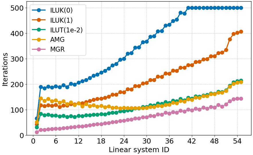
Linear solver iterations for different preconditioner configurations (Re=100, 256×256 grid).

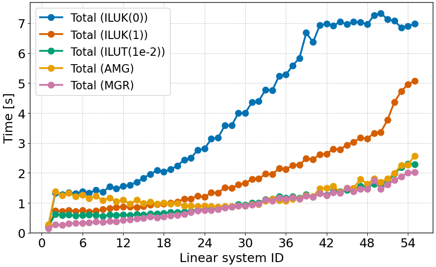
Total execution time for different preconditioner configurations (Re=100, 256×256 grid).

Time Stepping and Newton Convergence

The simulation advances in time using backward Euler with adaptive time stepping:

1. Initialize velocity and pressure to zero.

2. For each time step until final time:

   1. Perform Newton iterations until the residual norm is below tolerance.

   2. At each Newton iteration, assemble and solve the linearized system.

   3. Update the solution with the Newton correction.

   4. Optionally adjust \(\Delta t\) based on Newton convergence (adaptive stepping).

3. Write VTK output at specified intervals or at steady state.

The driver supports simple adaptive time stepping: if Newton converges quickly (≤3 iterations), \(\Delta t\) is increased; if convergence is slow (≥6 iterations), \(\Delta t\) is decreased. Additionally, a maximum CFL constraint can be specified using the -cfl option to prevent the time step from growing too large; when enabled, the time step is limited to \(\Delta t \leq \text{CFL}_{\max} \cdot h_{\min}\).

Visualizing the Solution

The driver outputs VTK RectilinearGrid files with velocity vectors, pressure, and divergence fields. A PVD collection file is written at the end to group all time steps for visualization in ParaView.

• -vis 1: Binary VTK, last time step only

• -vis 2: ASCII VTK, last time step only

• -vis 4: Binary VTK, all time steps

• -vis 6: ASCII VTK, all time steps

Output includes:

• velocity: 3-component vector field \((u, v, 0)\)

• pressure: Scalar field \(p\)

• div_velocity: Divergence \(\nabla \cdot \mathbf{u}\) (should be near zero)

Open the .pvd file in ParaView to visualize the flow evolution. Use “Stream Tracer” or “Glyph” filters to visualize the velocity field and vortex structures.

Validation Results

In this section, we validate the lid-driven cavity simulation by comparing 128×128 simulation centerline velocity profiles with high-resolution (8192×8192 grid) reference data from Marchi et al. (2021). The plots were generated using the postprocess.py script. They show the u-velocity profiles along the vertical centerline (x = 0.5) as a function of y and the v-velocity profiles along the horizontal centerline (y = 0.5) as a function of x. The error metrics (maximum error and RMSE) for both components are also displayed.

# Run test cases and plot centerlines comparison
./reproduce.sh --centerlines

# (Optional) Generate individual comparison plots (Re = 100)
python3 postprocess.py results.pvd --Re 100 --save lidcavity.png --compact

Centerline Velocity Profile Validation

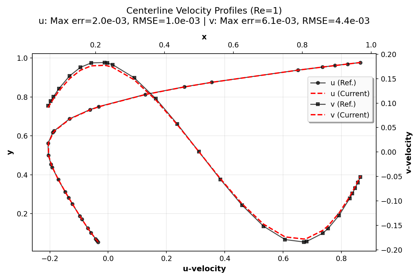
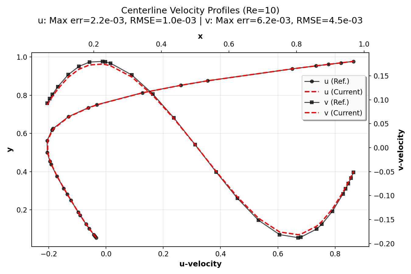
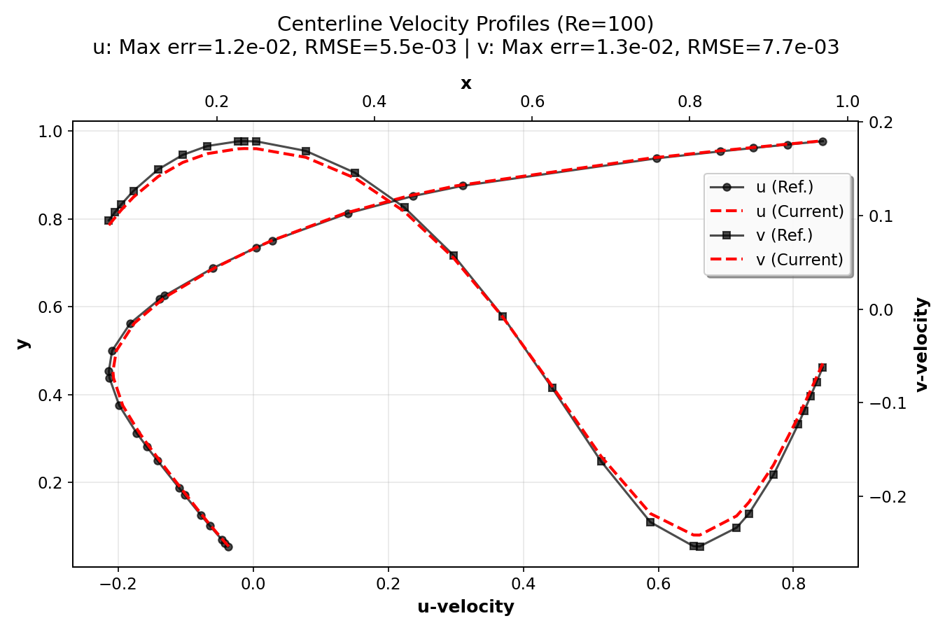
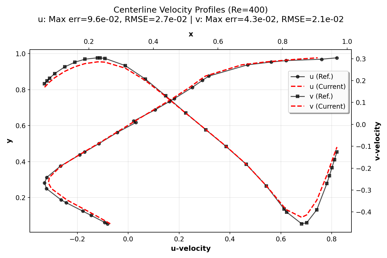
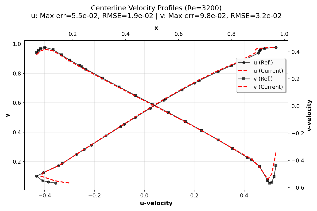
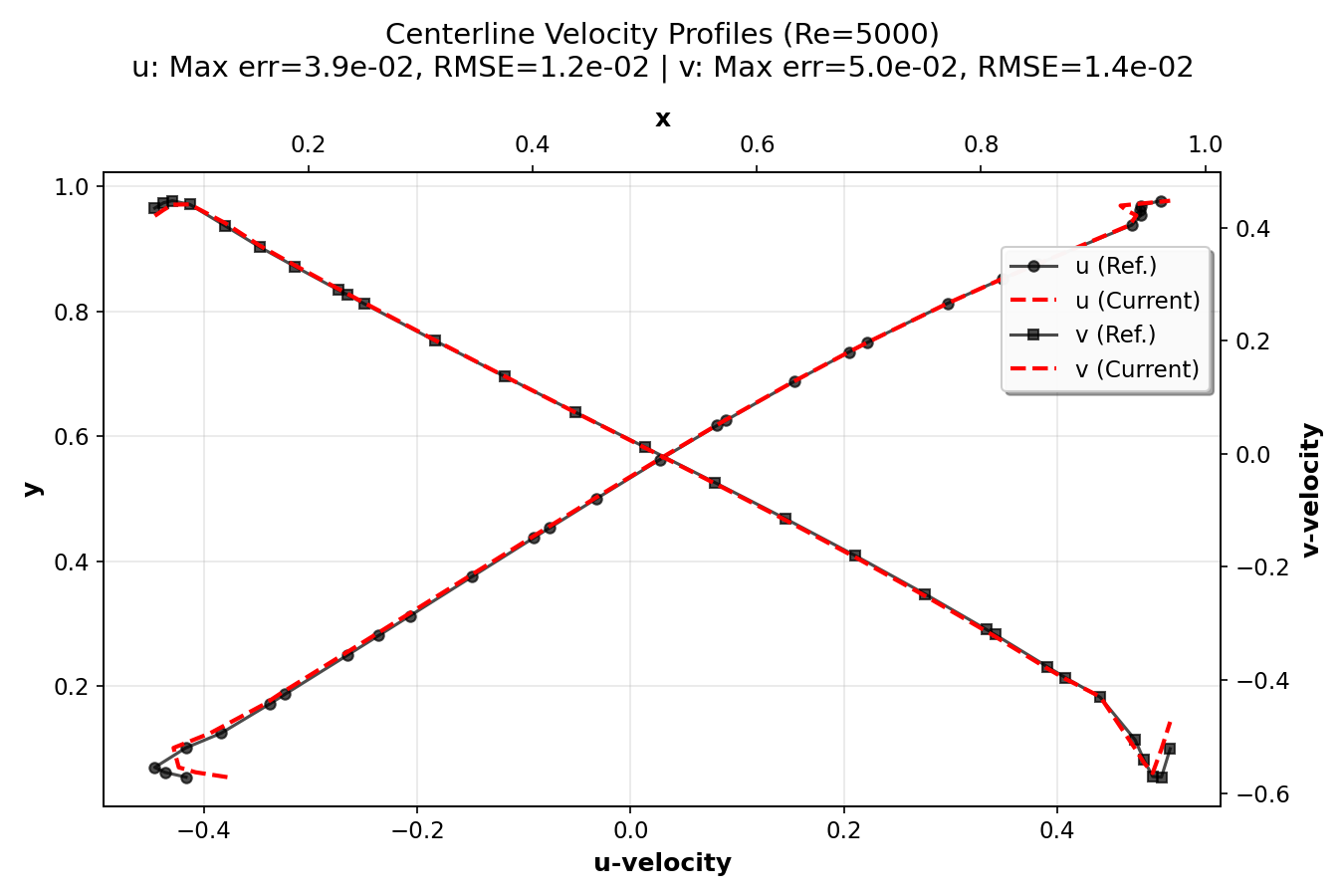
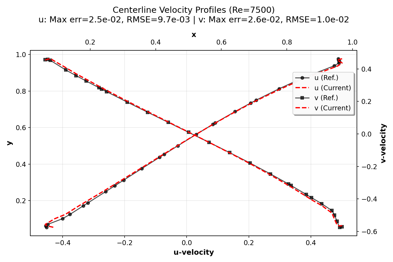
The validation demonstrates that the current numerical implementation provides accurate results across a wide range of Reynolds numbers, from creeping flow (Re = 1) to turbulent flow (Re = 7500). The agreement with high-resolution reference data (Marchi et al., 2021) confirms the correctness of the implementation. The compact plots show excellent agreement between simulation results and reference data, with error metrics (maximum error and RMSE) displayed for each Reynolds number.

Reproducible Run

Command-line parameters (see lidcavity -h) control problem size, Reynolds number, time stepping, partitioning, and visualization.

mpirun -np 1 /path/to/build/examples/src/C_lidcavity/lidcavity -h

Usage: ${MPIEXEC_COMMAND} <np> ./lidcavity [options]

Options:
  -i <file>         : YAML configuration file for solver settings (Opt.)
  -n <nx> <ny>      : Global grid dimensions in nodes (32 32)
  -P <Px> <Py>      : Processor grid dimensions (1 1)
  -L <Lx> <Ly>      : Physical dimensions (1 1)
  -Re <val>         : Reynolds number (100.0)
  -dt <val>         : Initial time step size (1)
  -tf <val>         : Final simulation time (50)
  -ntol <val>       : Non-linear solver tolerance (1.0e-6)
  -adt              : Enable simple adaptive time stepping
  -cfl <val>        : Maximum CFL for adaptive time stepping (0=no limit)
  -reg              : Use regularized lid BC (smooth corners)
  -br <n>           : Batch rows for matrix assembly (128)
  -vis <m>          : Visualization mode bitset (0)
                         Any nonzero value enables visualization
                         Bit 2 (0x2): ASCII (1) or binary (0)
                         Bit 3 (0x4): All timesteps (1) or last only (0)
  -v|--verbose <n>  : Verbosity bitset (0)
                         0x1: Linear solver statistics
                         0x2: Library information
                         0x4: Linear system printing
  -h|--help         : Print this message

Example run for Re=100 with visualization:

mpirun -np 1 /path/to/build/examples/src/C_lidcavity/lidcavity -vis 1

=====================================================
          Lid-Driven Cavity Problem Setup
=====================================================
Physical dimensions:     1 x 1
Grid dimensions (nodes): 32 x 32
Processor topology:      1 x 1
Reynolds number:         1.0e+02
Initial time step:       1.0e+00
Adaptive time stepping:  false
Regularized lid BC:      false
Final time:              5.0e+01
Visualization:           disabled
Verbosity level:         0x3
=====================================================

Date and time: 2026-02-06 00:30:13

Using HYPREDRV_DEVELOP_STRING: v0.1.0-60-g5785f920e (master)
Running on 1 MPI rank
------------------------------------------------------------------------------------
solver:
  fgmres:
    krylov_dim: 100
    max_iter: 300
    print_level: 0
    relative_tol: 1.0e-6
preconditioner:
  amg:
    print_level: 0
    coarsening:
      strong_th: 0.6
      num_functions: 3
    smoother:
      type: ilu
      num_levels: 5
      num_sweeps: 1
      ilu:
        type: bj-ilut
        fill_level: 0
        droptol: 1e-2
------------------------------------------------------------------------------------
Time step:   1 | Time: 1.0000e+00 [s] | CFL:    31.00 | NL:  1 | Lin:   2 | L2(u)=5.48e+00  L2(v)=0.00e+00  L2(p)=0.00e+00
Time step:   1 | Time: 1.0000e+00 [s] | CFL:    31.00 | NL:  2 | Lin:   3 | L2(u)=9.15e-03  L2(v)=3.41e-03  L2(p)=1.37e-02
Time step:   1 | Time: 1.0000e+00 [s] | CFL:    31.00 | NL:  3 | Lin:   3 | L2(u)=4.65e-04  L2(v)=3.74e-04  L2(p)=1.07e-03
Time step:   1 | Time: 1.0000e+00 [s] | CFL:    31.00 | NL:  4 | Lin:   2 | L2(u)=4.46e-05  L2(v)=3.36e-05  L2(p)=1.25e-04
Time step:   1 | Time: 1.0000e+00 [s] | CFL:    31.00 | NL:  5 | Lin:   3 | L2(u)=3.85e-06  L2(v)=5.05e-06  L2(p)=1.29e-05
Time step:   1 | Time: 1.0000e+00 [s] | CFL:    31.00 | NL:  6 | Lin:   3 | L2(u)=5.01e-07  L2(v)=8.04e-07  L2(p)=2.08e-06

Time step:   2 | Time: 2.0000e+00 [s] | CFL:    31.00 | NL:  1 | Lin:   4 | L2(u)=4.29e-03  L2(v)=2.35e-03  L2(p)=5.11e-04
Time step:   2 | Time: 2.0000e+00 [s] | CFL:    31.00 | NL:  2 | Lin:   4 | L2(u)=6.00e-04  L2(v)=5.65e-04  L2(p)=1.01e-03
Time step:   2 | Time: 2.0000e+00 [s] | CFL:    31.00 | NL:  3 | Lin:   3 | L2(u)=3.30e-05  L2(v)=3.70e-05  L2(p)=1.08e-04
Time step:   2 | Time: 2.0000e+00 [s] | CFL:    31.00 | NL:  4 | Lin:   3 | L2(u)=3.64e-06  L2(v)=5.79e-06  L2(p)=1.28e-05
Time step:   2 | Time: 2.0000e+00 [s] | CFL:    31.00 | NL:  5 | Lin:   3 | L2(u)=5.88e-07  L2(v)=1.02e-06  L2(p)=2.46e-06

Time step:   3 | Time: 3.0000e+00 [s] | CFL:    31.00 | NL:  1 | Lin:   4 | L2(u)=1.17e-03  L2(v)=9.62e-04  L2(p)=5.91e-05
Time step:   3 | Time: 3.0000e+00 [s] | CFL:    31.00 | NL:  2 | Lin:   4 | L2(u)=1.60e-04  L2(v)=1.81e-04  L2(p)=3.90e-04
Time step:   3 | Time: 3.0000e+00 [s] | CFL:    31.00 | NL:  3 | Lin:   3 | L2(u)=8.71e-06  L2(v)=9.82e-06  L2(p)=3.21e-05
Time step:   3 | Time: 3.0000e+00 [s] | CFL:    31.00 | NL:  4 | Lin:   3 | L2(u)=8.75e-07  L2(v)=1.32e-06  L2(p)=3.04e-06

Time step:   4 | Time: 4.0000e+00 [s] | CFL:    31.00 | NL:  1 | Lin:   4 | L2(u)=5.97e-04  L2(v)=5.24e-04  L2(p)=2.77e-05
Time step:   4 | Time: 4.0000e+00 [s] | CFL:    31.00 | NL:  2 | Lin:   4 | L2(u)=5.85e-05  L2(v)=7.18e-05  L2(p)=1.93e-04
Time step:   4 | Time: 4.0000e+00 [s] | CFL:    31.00 | NL:  3 | Lin:   3 | L2(u)=3.37e-06  L2(v)=3.53e-06  L2(p)=1.40e-05
Time step:   4 | Time: 4.0000e+00 [s] | CFL:    31.00 | NL:  4 | Lin:   3 | L2(u)=3.04e-07  L2(v)=3.92e-07  L2(p)=1.14e-06

Time step:   5 | Time: 5.0000e+00 [s] | CFL:    31.00 | NL:  1 | Lin:   4 | L2(u)=3.60e-04  L2(v)=3.16e-04  L2(p)=1.58e-05
Time step:   5 | Time: 5.0000e+00 [s] | CFL:    31.00 | NL:  2 | Lin:   4 | L2(u)=2.61e-05  L2(v)=3.26e-05  L2(p)=1.07e-04
Time step:   5 | Time: 5.0000e+00 [s] | CFL:    31.00 | NL:  3 | Lin:   3 | L2(u)=1.66e-06  L2(v)=1.66e-06  L2(p)=7.34e-06

Time step:   6 | Time: 6.0000e+00 [s] | CFL:    31.00 | NL:  1 | Lin:   4 | L2(u)=2.28e-04  L2(v)=2.01e-04  L2(p)=9.63e-06
Time step:   6 | Time: 6.0000e+00 [s] | CFL:    31.00 | NL:  2 | Lin:   4 | L2(u)=1.36e-05  L2(v)=1.64e-05  L2(p)=6.32e-05
Time step:   6 | Time: 6.0000e+00 [s] | CFL:    31.00 | NL:  3 | Lin:   3 | L2(u)=9.53e-07  L2(v)=9.10e-07  L2(p)=4.20e-06

Time step:   7 | Time: 7.0000e+00 [s] | CFL:    31.00 | NL:  1 | Lin:   4 | L2(u)=1.48e-04  L2(v)=1.31e-04  L2(p)=6.00e-06
Time step:   7 | Time: 7.0000e+00 [s] | CFL:    31.00 | NL:  2 | Lin:   4 | L2(u)=7.92e-06  L2(v)=9.02e-06  L2(p)=3.88e-05
Time step:   7 | Time: 7.0000e+00 [s] | CFL:    31.00 | NL:  3 | Lin:   3 | L2(u)=5.94e-07  L2(v)=5.41e-07  L2(p)=2.52e-06

Time step:   8 | Time: 8.0000e+00 [s] | CFL:    31.00 | NL:  1 | Lin:   4 | L2(u)=9.63e-05  L2(v)=8.60e-05  L2(p)=3.81e-06
Time step:   8 | Time: 8.0000e+00 [s] | CFL:    31.00 | NL:  2 | Lin:   4 | L2(u)=4.94e-06  L2(v)=5.26e-06  L2(p)=2.44e-05
Time step:   8 | Time: 8.0000e+00 [s] | CFL:    31.00 | NL:  3 | Lin:   3 | L2(u)=3.84e-07  L2(v)=3.34e-07  L2(p)=1.56e-06

Time step:   9 | Time: 9.0000e+00 [s] | CFL:    31.00 | NL:  1 | Lin:   4 | L2(u)=6.29e-05  L2(v)=5.67e-05  L2(p)=2.44e-06
Time step:   9 | Time: 9.0000e+00 [s] | CFL:    31.00 | NL:  2 | Lin:   4 | L2(u)=3.17e-06  L2(v)=3.20e-06  L2(p)=1.55e-05
Time step:   9 | Time: 9.0000e+00 [s] | CFL:    31.00 | NL:  3 | Lin:   3 | L2(u)=2.51e-07  L2(v)=2.11e-07  L2(p)=9.81e-07

Time step:  10 | Time: 1.0000e+01 [s] | CFL:    31.00 | NL:  1 | Lin:   4 | L2(u)=4.10e-05  L2(v)=3.73e-05  L2(p)=1.57e-06
Time step:  10 | Time: 1.0000e+01 [s] | CFL:    31.00 | NL:  2 | Lin:   4 | L2(u)=2.06e-06  L2(v)=1.99e-06  L2(p)=9.94e-06

Time step:  11 | Time: 1.1000e+01 [s] | CFL:    31.00 | NL:  1 | Lin:   4 | L2(u)=2.68e-05  L2(v)=2.45e-05  L2(p)=1.32e-06
Time step:  11 | Time: 1.1000e+01 [s] | CFL:    31.00 | NL:  2 | Lin:   4 | L2(u)=1.34e-06  L2(v)=1.27e-06  L2(p)=6.41e-06

Time step:  12 | Time: 1.2000e+01 [s] | CFL:    31.00 | NL:  1 | Lin:   4 | L2(u)=1.74e-05  L2(v)=1.60e-05  L2(p)=8.37e-07
Time step:  12 | Time: 1.2000e+01 [s] | CFL:    31.00 | NL:  2 | Lin:   4 | L2(u)=8.77e-07  L2(v)=8.10e-07  L2(p)=4.14e-06

Time step:  13 | Time: 1.3000e+01 [s] | CFL:    31.00 | NL:  1 | Lin:   4 | L2(u)=1.14e-05  L2(v)=1.05e-05  L2(p)=5.42e-07
Time step:  13 | Time: 1.3000e+01 [s] | CFL:    31.00 | NL:  2 | Lin:   4 | L2(u)=5.72e-07  L2(v)=5.21e-07  L2(p)=2.68e-06

Time step:  14 | Time: 1.4000e+01 [s] | CFL:    31.00 | NL:  1 | Lin:   4 | L2(u)=7.39e-06  L2(v)=6.83e-06  L2(p)=3.51e-07
Time step:  14 | Time: 1.4000e+01 [s] | CFL:    31.00 | NL:  2 | Lin:   4 | L2(u)=3.72e-07  L2(v)=3.37e-07  L2(p)=1.74e-06

Time step:  15 | Time: 1.5000e+01 [s] | CFL:    31.00 | NL:  1 | Lin:   4 | L2(u)=4.81e-06  L2(v)=4.45e-06  L2(p)=2.28e-07
Time step:  15 | Time: 1.5000e+01 [s] | CFL:    31.00 | NL:  2 | Lin:   4 | L2(u)=2.42e-07  L2(v)=2.18e-07  L2(p)=1.13e-06

Time step:  16 | Time: 1.6000e+01 [s] | CFL:    31.00 | NL:  1 | Lin:   4 | L2(u)=3.13e-06  L2(v)=2.89e-06  L2(p)=1.48e-07
Time step:  17 | Time: 1.8000e+01 [s] | CFL:    62.00 | NL:  1 | Lin:   3 | L2(u)=6.17e-06  L2(v)=7.66e-06  L2(p)=3.78e-05
Time step:  17 | Time: 1.8000e+01 [s] | CFL:    62.00 | NL:  2 | Lin:   3 | L2(u)=1.97e-06  L2(v)=1.44e-06  L2(p)=6.10e-06

Time step:  18 | Time: 2.0000e+01 [s] | CFL:    62.00 | NL:  1 | Lin:   4 | L2(u)=1.18e-06  L2(v)=9.41e-07  L2(p)=5.80e-07
Time step:  19 | Time: 2.4000e+01 [s] | CFL:   124.00 | NL:  1 | Lin:   3 | L2(u)=1.54e-06  L2(v)=1.89e-06  L2(p)=9.52e-06
Time step:  19 | Time: 2.4000e+01 [s] | CFL:   124.00 | NL:  2 | Lin:   3 | L2(u)=4.98e-07  L2(v)=3.63e-07  L2(p)=1.54e-06

Time step:  20 | Time: 2.8000e+01 [s] | CFL:   124.00 | NL:  1 | Lin:   4 | L2(u)=1.64e-07  L2(v)=1.38e-07  L2(p)=1.65e-07
Time step:  21 | Time: 3.6000e+01 [s] | CFL:   248.00 | NL:  1 | Lin:   4 | L2(u)=3.70e-07  L2(v)=4.63e-07  L2(p)=2.38e-06
Time step:  22 | Time: 5.0000e+01 [s] | CFL:   434.00 | NL:  1 | Lin:   3 | L2(u)=1.64e-07  L2(v)=1.27e-07  L2(p)=7.51e-07

Aggregate Summary:
--------------------------------------------------------------
Total number of Non-linear iterations: 55
Total number of linear iterations:     148
Avg. LS iterations:                    2.69
Avg. LS times: (setup, solve, total):  0.0283, 0.0017, 0.0300
Total LS times: (setup, solve, total): 1.5564, 0.0921, 1.6485
Avg. LS iterations per timestep:       6.73
Avg. LS times per timestep: (s, s, t): 0.0707, 0.0042, 0.0749
--------------------------------------------------------------

====================================================================================


STATISTICS SUMMARY:

+---------+-------------+-------------+-------------+------------+------------+---------+
|         |    LS build |       setup |       solve |    initial |   relative |         |
|   Entry |   times [s] |   times [s] |   times [s] |  res. norm |  res. norm |   iters |
+---------+-------------+-------------+-------------+------------+------------+---------+
|       0 |       0.001 |       0.023 |       0.001 |   5.48e+00 |   4.79e-08 |       2 |
|       1 |       0.001 |       0.032 |       0.002 |   1.68e-02 |   4.20e-07 |       3 |
|       2 |       0.001 |       0.033 |       0.002 |   1.22e-03 |   4.06e-07 |       3 |
|       3 |       0.001 |       0.033 |       0.001 |   1.37e-04 |   8.82e-07 |       2 |
|       4 |       0.001 |       0.032 |       0.002 |   1.44e-05 |   1.72e-07 |       3 |
|       5 |       0.001 |       0.032 |       0.002 |   2.28e-06 |   1.16e-07 |       3 |
|       6 |       0.001 |       0.032 |       0.002 |   4.92e-03 |   6.96e-09 |       4 |
|       7 |       0.001 |       0.035 |       0.003 |   1.31e-03 |   3.99e-09 |       4 |
|       8 |       0.001 |       0.035 |       0.002 |   1.19e-04 |   4.51e-07 |       3 |
|       9 |       0.001 |       0.035 |       0.002 |   1.45e-05 |   4.68e-07 |       3 |
|      10 |       0.001 |       0.035 |       0.002 |   2.72e-06 |   2.30e-07 |       3 |
|      11 |       0.001 |       0.035 |       0.002 |   1.51e-03 |   3.40e-08 |       4 |
|      12 |       0.001 |       0.036 |       0.002 |   4.59e-04 |   8.06e-09 |       4 |
|      13 |       0.001 |       0.037 |       0.002 |   3.47e-05 |   6.58e-07 |       3 |
|      14 |       0.001 |       0.037 |       0.002 |   3.43e-06 |   3.01e-07 |       3 |
|      15 |       0.001 |       0.037 |       0.003 |   7.95e-04 |   5.41e-08 |       4 |
|      16 |       0.001 |       0.037 |       0.002 |   2.14e-04 |   8.17e-09 |       4 |
|      17 |       0.001 |       0.037 |       0.002 |   1.48e-05 |   2.13e-07 |       3 |
|      18 |       0.001 |       0.037 |       0.002 |   1.24e-06 |   3.11e-07 |       3 |
|      19 |       0.001 |       0.037 |       0.003 |   4.79e-04 |   2.89e-08 |       4 |
|      20 |       0.001 |       0.038 |       0.002 |   1.15e-04 |   1.31e-08 |       4 |
|      21 |       0.001 |       0.038 |       0.002 |   7.71e-06 |   7.82e-07 |       3 |
|      22 |       0.001 |       0.038 |       0.002 |   3.04e-04 |   6.71e-08 |       4 |
|      23 |       0.001 |       0.038 |       0.003 |   6.67e-05 |   1.55e-08 |       4 |
|      24 |       0.001 |       0.038 |       0.002 |   4.40e-06 |   9.63e-07 |       3 |
|      25 |       0.001 |       0.039 |       0.002 |   1.97e-04 |   7.07e-08 |       4 |
|      26 |       0.001 |       0.040 |       0.003 |   4.06e-05 |   1.57e-08 |       4 |
|      27 |       0.001 |       0.039 |       0.002 |   2.65e-06 |   9.02e-07 |       3 |
|      28 |       0.001 |       0.040 |       0.002 |   1.29e-04 |   6.57e-08 |       4 |
|      29 |       0.001 |       0.040 |       0.002 |   2.54e-05 |   1.86e-08 |       4 |
|      30 |       0.001 |       0.040 |       0.002 |   1.64e-06 |   9.80e-07 |       3 |
|      31 |       0.001 |       0.040 |       0.003 |   8.47e-05 |   6.07e-08 |       4 |
|      32 |       0.001 |       0.040 |       0.003 |   1.62e-05 |   1.84e-08 |       4 |
|      33 |       0.002 |       0.040 |       0.002 |   1.03e-06 |   9.32e-07 |       3 |
|      34 |       0.001 |       0.041 |       0.003 |   5.55e-05 |   4.87e-08 |       4 |
|      35 |       0.001 |       0.040 |       0.003 |   1.03e-05 |   1.15e-08 |       4 |
|      36 |       0.001 |       0.040 |       0.002 |   3.63e-05 |   3.63e-08 |       4 |
|      37 |       0.001 |       0.041 |       0.003 |   6.67e-06 |   1.15e-08 |       4 |
|      38 |       0.001 |       0.042 |       0.003 |   2.37e-05 |   3.36e-08 |       4 |
|      39 |       0.001 |       0.039 |       0.003 |   4.31e-06 |   1.34e-08 |       4 |
|      40 |       0.001 |       0.039 |       0.002 |   1.55e-05 |   3.99e-08 |       4 |
|      41 |       0.001 |       0.039 |       0.003 |   2.79e-06 |   2.07e-08 |       4 |
|      42 |       0.001 |       0.039 |       0.002 |   1.01e-05 |   6.34e-08 |       4 |
|      43 |       0.001 |       0.038 |       0.003 |   1.81e-06 |   2.05e-08 |       4 |
|      44 |       0.001 |       0.039 |       0.002 |   6.56e-06 |   6.87e-08 |       4 |
|      45 |       0.001 |       0.039 |       0.002 |   1.17e-06 |   1.90e-08 |       4 |
|      46 |       0.001 |       0.039 |       0.002 |   4.27e-06 |   6.26e-08 |       4 |
|      47 |       0.001 |       0.041 |       0.002 |   3.91e-05 |   7.94e-07 |       3 |
|      48 |       0.002 |       0.041 |       0.002 |   6.57e-06 |   4.59e-07 |       3 |
|      49 |       0.001 |       0.040 |       0.003 |   1.62e-06 |   2.94e-07 |       4 |
|      50 |       0.001 |       0.043 |       0.002 |   9.83e-06 |   9.81e-07 |       3 |
|      51 |       0.001 |       0.041 |       0.002 |   1.66e-06 |   7.67e-07 |       3 |
|      52 |       0.001 |       0.042 |       0.002 |   2.71e-07 |   9.65e-07 |       4 |
|      53 |       0.001 |       0.043 |       0.002 |   2.45e-06 |   9.37e-08 |       4 |
|      54 |       0.001 |       0.044 |       0.002 |   7.79e-07 |   9.92e-07 |       3 |
+---------+-------------+-------------+-------------+------------+------------+---------+

Date and time: 2026-02-06 00:30:16
lidcavity done!

The transient streamlines can be rendered as an animated GIF with the postprocess.py script, which traces the velocity field at each timestep using PyVista (write all timesteps with -vis 4):

mpirun -np 4 /path/to/build/lidcavity -n 96 96 -P 2 2 -Re 100 -dt 0.05 -tf 50 -adt -reg -vis 4 -i fgmres-ilu0.yml
python3 postprocess.py lidcavity_Re100_96x96_2x2.pvd --Re 100 --video lidcavity_streamlines.gif   # needs: pip install pyvista imageio

Streamlines of the lid-driven cavity flow (Re=100) over the transient, colored by the velocity magnitude. The primary vortex forms and the two secondary corner eddies emerge as the flow approaches steady state.

Example 6: Definite curl-curl (AMS)

This example, implemented in examples/src/C_maxwell/maxwell.c, is an electromagnetic benchmark for the Auxiliary-space Maxwell Solver (AMS). It pairs a lowest-order edge-element discretization of a definite Maxwell problem with a manufactured solution, so that both the algebraic performance (iteration counts, timings) and the discretization accuracy can be measured directly.

Governing Equations (Definite Maxwell)

On a box \(\Omega=[0,L_x]\times[0,L_y]\times[0,L_z]\) we solve the curl-curl + mass (also called definite Maxwell) problem for the electric field \(E\):

\[\nabla\times\!\big(\mu^{-1}\,\nabla\times E\big) + \sigma\,E = f \quad\text{in } \Omega, \qquad E\times n = (E\times n)_D \quad\text{on } \partial\Omega ,\]

where \(\mu^{-1}\) is the inverse magnetic permeability (the curl-curl coefficient) and \(\sigma\ge 0\) is the conductivity / mass coefficient. Both default to \(1\) and are configurable with the -muinv and -sigma flags. The essential boundary condition prescribes the tangential trace \(E\times n\), which is the natural Dirichlet datum for fields in \(H(\mathrm{curl})\).

The mass term is what makes the operator definite: for \(\sigma>0\) the bilinear form is coercive on all of \(H(\mathrm{curl})\) (the gradient fields, which lie in the kernel of the curl, are controlled by the \(\sigma\,E\) term). This is exactly the regime AMS is designed for, and AMS remains robust across the whole range from curl-dominated (\(\sigma\ll\mu^{-1}\)) to mass-dominated (\(\sigma\gg\mu^{-1}\)) as long as \(\sigma\ge 0\).

Variational Formulation

Let \(V=\{v\in H(\mathrm{curl};\Omega): v\times n=0 \text{ on }\partial\Omega\}\). The weak problem reads: find \(E\in E_D+V\) such that for all \(v\in V\),

\[\int_\Omega \mu^{-1}\,(\nabla\times E)\cdot(\nabla\times v)\,d\Omega \;+\; \int_\Omega \sigma\,E\cdot v\,d\Omega \;=\; \int_\Omega f\cdot v\,d\Omega .\]

The two volume integrals give, after discretization, a stiffness (curl-curl) matrix weighted by \(\mu^{-1}\) and a mass matrix weighted by \(\sigma\); the system matrix is their sum.

Discretization: Lowest-Order Nedelec (Edge) Elements

The field is discretized with the lowest-order Nedelec (Whitney) edge elements on a structured hexahedral mesh. The degrees of freedom live on edges: the DOF of edge \(e\) is the integral of the tangential component of \(E\) along it,

\[\mathrm{dof}_e(E) \;=\; \int_e E\cdot \tau \, ds ,\]

with every edge oriented in the \(+\)-axis direction. Each hexahedron carries 12 edge DOFs (four per axis direction). The example builds the \(12\times12\) element matrix \(S_K = \mu^{-1}\,K_K + \sigma\,M_K\) by integrating the Whitney basis with a \(3\)-point Gauss rule per direction, where \((K_K)_{ab}=\int_K(\nabla\times W_a)\cdot(\nabla\times W_b)\) and \((M_K)_{ab}=\int_K W_a\cdot W_b\). The essential boundary condition is imposed by element-level static condensation: boundary-edge rows become identity rows whose right-hand side is the prescribed tangential value, and their columns are lifted to the load of the interior rows.

Nodes, edges, and (for the H(div) example below) faces are numbered with a single rank-monotonic scheme so that the node, edge, and face partitions are mutually consistent – a requirement for the auxiliary-space products formed internally by AMS and ADS.

Manufactured Solution and Error Measurement

The benchmark uses the smooth field

\[E=(\sin\kappa y,\ \sin\kappa z,\ \sin\kappa x),\qquad \kappa=\text{freq}\cdot\pi \ \ (\texttt{-freq}, \text{ default } 1),\]

which is an eigenfunction of the curl-curl operator: a short computation gives \(\nabla\times E=(-\kappa\cos\kappa z,-\kappa\cos\kappa x,-\kappa\cos\kappa y)\) and hence \(\nabla\times\nabla\times E=\kappa^2 E\). The forcing is therefore available in closed form,

\[f \;=\; \mu^{-1}\,\nabla\times\nabla\times E + \sigma\,E \;=\; (\mu^{-1}\kappa^2+\sigma)\,E ,\]

and the exact edge DOFs reduce to one-dimensional integrals, e.g. for an \(x\)-edge at nodal height \(y\) the DOF is \(h_x\sin(\kappa y)\). After the solve the example compares the computed edge DOFs to this reference field and reports the relative discrete \(\ell_2\) error, which confirms the solver converges to the correct field rather than merely to a small residual.

Auxiliary-Space Inputs: the Discrete de Rham Complex

AMS accelerates the edge system by mapping curl-free error components into nodal (\(H^1\)) auxiliary spaces, where standard AMG is effective. This requires two operator inputs beyond the system matrix, both reflecting the de Rham complex \(H^1 \xrightarrow{\nabla} H(\mathrm{curl}) \xrightarrow{\nabla\times} H(\mathrm{div})\):

• the discrete gradient \(G\) (an edge \(\times\) node incidence matrix with entries \(-1\) at the tail node and \(+1\) at the head node of each edge), passed with HYPREDRV_LinearSystemSetDiscreteGradient(); and

• the vertex coordinate vectors \(x,y,z\), passed with HYPREDRV_LinearSystemSetCoordinates().

The example assembles \(G\) as an HYPRE_IJMatrix (edges \(\times\) nodes) and the coordinates as three nodal HYPRE_IJVector objects. Note that these inputs are purely topological/geometric: they do not depend on \(\mu^{-1}\) or \(\sigma\).

Linear System Creation

The driver builds the IJ objects itself and hands them to HYPREDRV in library mode:

HYPREDRV_LinearSystemSetMatrix(hypredrv, (HYPRE_Matrix) A);
HYPREDRV_LinearSystemSetRHS(hypredrv, (HYPRE_Vector) b);
HYPREDRV_LinearSystemSetDiscreteGradient(hypredrv, (HYPRE_Matrix) G);
HYPREDRV_LinearSystemSetCoordinates(hypredrv,
                                    (HYPRE_Vector) xcoord,
                                    (HYPRE_Vector) ycoord,
                                    (HYPRE_Vector) zcoord);

The solver and preconditioner are configured from examples/src/C_maxwell/pcg-ams.yml (PCG + AMS). A typical run:

mpirun -np 4 /path/to/build/maxwell -i pcg-ams.yml -n 33 33 33 -P 2 2 1

Solution Visualization

Passing -vtk <base> writes the computed field as VTK ImageData – a single <base>.vti on one rank, or a <base>.pvti master plus per-rank <base>_pN.vti pieces in parallel. The driver reconstructs the cell-centered electric field from the edge DOFs (Whitney basis) and stores both the vector and its magnitude. The bundled postprocess.py renders the magnitude with PyVista; by default it draws nested translucent isosurfaces (level sets) that show the 3D structure of the field. The --style flag also offers clip (octant cutaway), volume (volume rendering), and slices:

mpirun -np 4 /path/to/build/maxwell -i pcg-ams.yml -n 65 65 65 -P 2 2 1 -vtk maxwell
python3 postprocess.py maxwell.pvti -o maxwell_solution_3d.png   # needs: pip install pyvista

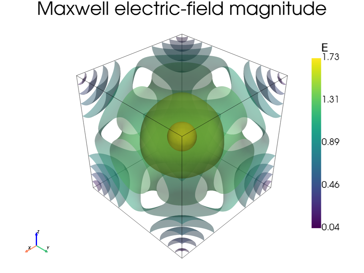
Computed electric-field magnitude \(\|E\|_2\) on a \(64^3\) mesh (4 MPI ranks) for the default manufactured solution (\(\text{freq}=1\)), shown as nested isosurfaces. The field is smooth and peaks at the cube center. The same .vti/.pvti files can also be opened directly in ParaView.

Mesh Refinement (Discretization Accuracy)

./reproduce.sh (the default refine mode) confirms convergence to the manufactured field. AMS keeps the iteration count nearly mesh independent while the discrete \(\ell_2\) error drops like \(O(h^2)\):

grid       iters        rel. error
9^3        4            5.302372e-04
17^3       7            1.358464e-04
33^3       9            3.443534e-05
65^3       10           8.673237e-06

Coefficient Robustness

The ./reproduce.sh sweep mode probes robustness with respect to the coefficients on the \(64^3\) mesh (~0.8M edge unknowns). Because the discrete operator is \(\mu^{-1}K+\sigma M\), what matters is the curl-to-mass ratio \(\sigma/\mu^{-1}\), so it suffices to fix \(\mu^{-1}=1\) and sweep \(\sigma\) over six orders of magnitude, \(\sigma\in\{10^{-3},\dots,10^{3}\}\): values below 1 are curl-dominated and values above 1 are mass-dominated. The iteration plot compares AMS against two generic preconditioners that are not tailored to \(H(\mathrm{curl})\) – BoomerAMG (pcg-amg.yml) and restricted additive Schwarz with one level of overlap and ILU(0) subdomain solves (gmres-ras1-ilu0.yml) – all driven to relative_tol = 1e-8 with a cap of 500 iterations.

cd /path/to/build/examples/src/C_maxwell
MPI_RANKS=4 PGRID="2 2 1" ./reproduce.sh sweep

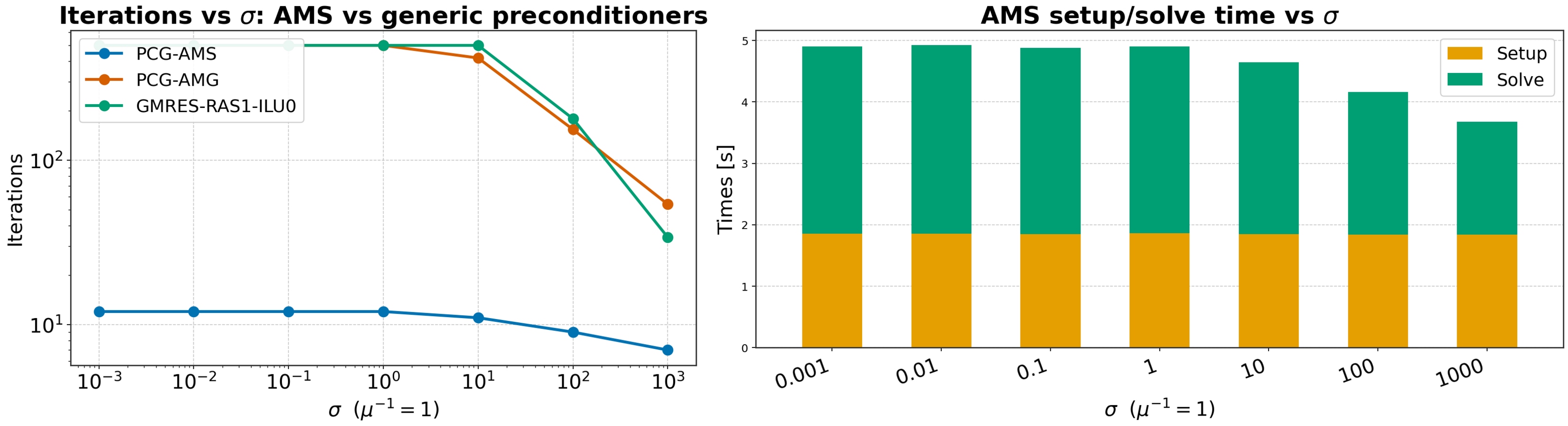
Definite Maxwell problem on a \(64^3\) mesh (4 MPI ranks). Left: iteration count versus \(\sigma\) (log-log) for AMS, BoomerAMG, and RAS(1)-ILU0. Right: stacked AMS setup/solve time versus \(\sigma\).

The contrast is stark. AMS is flat and robust: 12 iterations in the curl-dominated regime, easing to 7 as the mass term makes the system better conditioned – essentially independent of \(\sigma\). The generic preconditioners, by contrast, fail in the curl-dominated regime: both BoomerAMG and RAS(1)-ILU0 hit the 500-iteration cap for small \(\sigma\) (BoomerAMG for \(\sigma\le 1\), RAS for \(\sigma\le 10\)), and recover only once the mass term dominates (\(\sigma\gtrsim 100\)), where the matrix approaches a well-conditioned mass matrix and any reasonable smoother works. This is exactly why an auxiliary-space solver is needed: only AMS handles the large near-kernel of the curl operator. Finally, the AMS setup time is independent of \(\sigma\) (~2 s throughout), because the auxiliary-space hierarchy is built from the discrete gradient and the vertex coordinates – the problem topology and geometry – not from the coefficient values; the solve time simply tracks the iteration count.

Note

The comparison uses 4 MPI ranks because, in the bundled HYPRE build, the overlapping Schwarz (RAS) setup aborts at higher rank counts on this \(64^3\) system; AMS, ADS, and BoomerAMG run at any rank count.

Example 7: Definite grad-div (ADS)

This example, in examples/src/C_graddiv/graddiv.c, is the \(H(\mathrm{div})\) counterpart of the Maxwell benchmark and targets the Auxiliary-space Divergence Solver (ADS). It mirrors Example 6 one step down the de Rham complex: edges become faces, the curl-curl operator becomes grad-div, and Nedelec elements become Raviart-Thomas elements.

Governing Equations (Definite grad-div)

On a box \(\Omega\) we solve the grad-div + mass problem for a vector field \(u\) (a flux/velocity):

\[-\alpha\,\nabla(\nabla\cdot u) + \beta\,u = f \quad\text{in } \Omega, \qquad u\cdot n = (u\cdot n)_D \quad\text{on } \partial\Omega ,\]

where \(\alpha\) weights the grad-div (divergence-stiffness) term and \(\beta\ge 0\) is the mass coefficient; both default to \(1\) and are set with -alpha and -beta. The essential boundary condition prescribes the normal trace \(u\cdot n\), the natural Dirichlet datum in \(H(\mathrm{div})\). As before the mass term makes the operator definite (it controls the divergence-free fields that lie in the kernel of the divergence), which is the regime ADS is built for.

Variational Formulation

With \(W=\{v\in H(\mathrm{div};\Omega): v\cdot n=0\text{ on }\partial\Omega\}\), the weak form is: find \(u\in u_D+W\) such that for all \(v\in W\),

\[\int_\Omega \alpha\,(\nabla\cdot u)(\nabla\cdot v)\,d\Omega \;+\; \int_\Omega \beta\,u\cdot v\,d\Omega \;=\; \int_\Omega f\cdot v\,d\Omega ,\]

giving a divergence-stiffness matrix weighted by \(\alpha\) plus a mass matrix weighted by \(\beta\).

Discretization: Lowest-Order Raviart-Thomas (Face) Elements

The flux is discretized with lowest-order Raviart-Thomas (RT0) face elements. The degrees of freedom live on faces: the DOF of face \(F\) is the integral of the normal flux through it,

\[\mathrm{dof}_F(u) \;=\; \int_F u\cdot n \, dA ,\]

with every face normal oriented in the \(+\)-axis direction. Each hexahedron carries 6 face DOFs. The \(6\times6\) element matrix \(S_K=\alpha\,K^{\mathrm{div}}_K + \beta\,M_K\) is integrated from the RT0 basis, with \((K^{\mathrm{div}}_K)_{ab}=\int_K(\nabla\cdot v_a)(\nabla\cdot v_b)\) and \((M_K)_{ab}=\int_K v_a\cdot v_b\). The normal-trace boundary condition is imposed by the same element-level static condensation used in the Maxwell example.

Manufactured Solution and Error Measurement

The benchmark uses

\[u=(\sin\kappa x,\ \sin\kappa y,\ \sin\kappa z),\qquad \kappa=\text{freq}\cdot\pi .\]

Here \(\nabla\cdot u=\kappa(\cos\kappa x+\cos\kappa y+\cos\kappa z)\) and \(\nabla(\nabla\cdot u)=-\kappa^2 u\), so the forcing is again closed-form,

\[f \;=\; -\alpha\,\nabla(\nabla\cdot u)+\beta\,u \;=\; (\alpha\kappa^2+\beta)\,u ,\]

and the exact face DOFs reduce to surface integrals such as \(h_y h_z\sin(\kappa x)\) for an \(x\)-face. The example reports the relative discrete \(\ell_2\) error of the computed face DOFs against this reference.

Auxiliary-Space Inputs: the Full de Rham Complex

ADS reduces the face system through the edge space (where it applies AMS) and then to the nodal space. It therefore needs the whole discrete de Rham sequence \(\text{nodes}\xrightarrow{G}\text{edges}\xrightarrow{C}\text{faces}\), i.e. three operator inputs in addition to the system matrix:

• the discrete gradient \(G\) (edge \(\times\) node), via HYPREDRV_LinearSystemSetDiscreteGradient();

• the discrete curl \(C\) (face \(\times\) edge incidence, with right-hand-rule signs around each face), via HYPREDRV_LinearSystemSetDiscreteCurl(); and

• the vertex coordinate vectors, via HYPREDRV_LinearSystemSetCoordinates().

The example constructs \(G\) and \(C\) so that the fundamental identity \(C\,G=0\) (the discrete curl of a gradient is zero) holds exactly – a property ADS relies on. As in the Maxwell case these inputs are purely topological/geometric and independent of \(\alpha\) and \(\beta\).

Linear System Creation

HYPREDRV_LinearSystemSetMatrix(hypredrv, (HYPRE_Matrix) A);
HYPREDRV_LinearSystemSetRHS(hypredrv, (HYPRE_Vector) b);
HYPREDRV_LinearSystemSetDiscreteGradient(hypredrv, (HYPRE_Matrix) G);
HYPREDRV_LinearSystemSetDiscreteCurl(hypredrv, (HYPRE_Matrix) C);
HYPREDRV_LinearSystemSetCoordinates(hypredrv,
                                    (HYPRE_Vector) xcoord,
                                    (HYPRE_Vector) ycoord,
                                    (HYPRE_Vector) zcoord);

The solver/preconditioner come from examples/src/C_graddiv/pcg-ads.yml (PCG + ADS):

mpirun -np 4 /path/to/build/graddiv -i pcg-ads.yml -n 33 33 33 -P 2 2 1

Solution Visualization

As in the Maxwell example, -vtk <base> writes the solution as VTK ImageData (serial <base>.vti or parallel <base>.pvti plus per-rank pieces); here the cell-centered flux is reconstructed from the face DOFs using the RT0 basis. The bundled postprocess.py renders the magnitude with PyVista, using the same isosurface default (and the same --style options) as the Maxwell example:

mpirun -np 4 /path/to/build/graddiv -i pcg-ads.yml -n 65 65 65 -P 2 2 1 -freq 2 -vtk graddiv
python3 postprocess.py graddiv.pvti -o graddiv_solution_3d.png   # needs: pip install pyvista

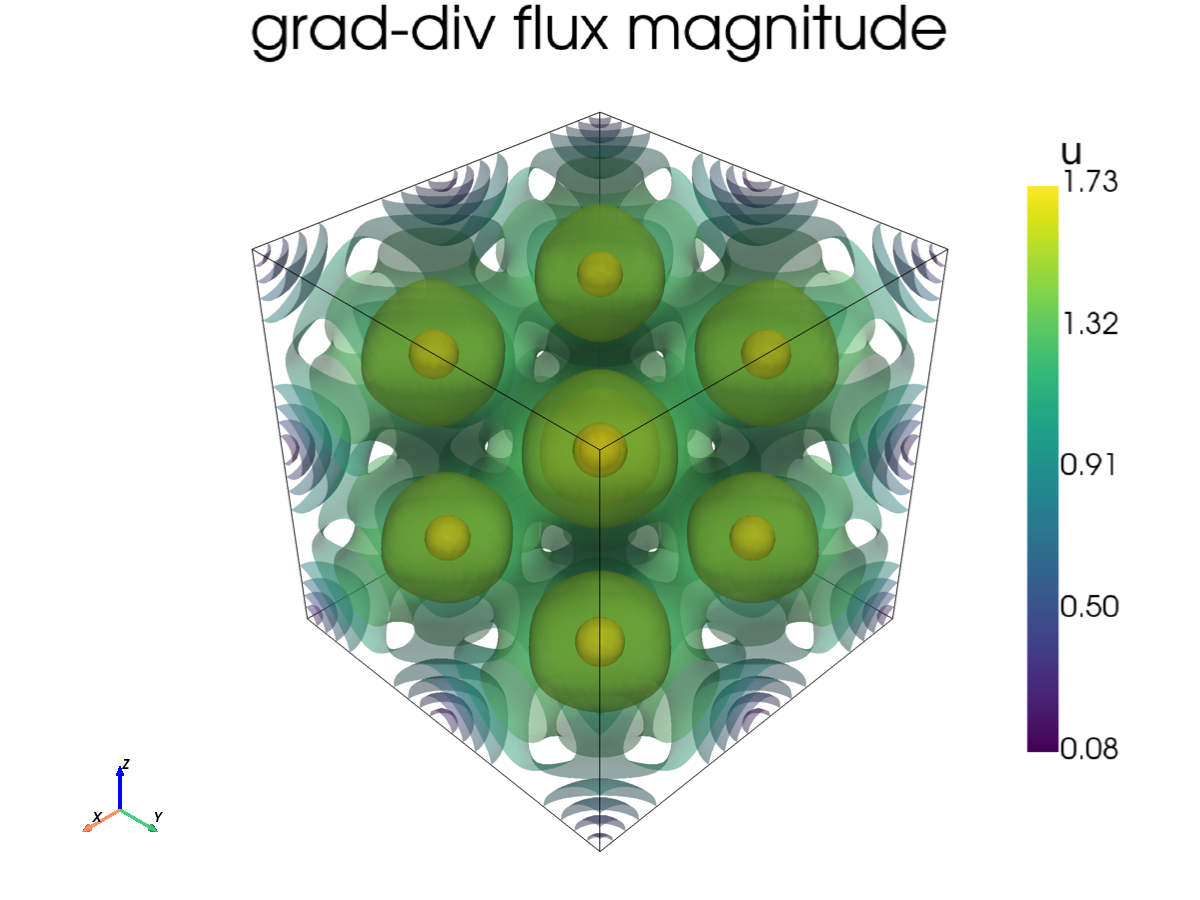
Computed flux magnitude \(\|u\|_2\) on a \(64^3\) mesh (4 MPI ranks) for the manufactured solution at frequency -freq 2 (\(\kappa = 2\pi\)), shown as nested isosurfaces. The higher frequency produces a periodic lattice of peaks throughout the domain, so the field looks visibly different from the single central peak of the Maxwell example (which uses the default -freq 1).

Mesh Refinement (Discretization Accuracy)

./reproduce.sh shows ADS behaving like AMS – nearly mesh independent with \(O(h^2)\) error decay:

grid       iters        rel. error
9^3        5            1.174488e-03
17^3       8            2.950893e-04
33^3       10           7.386281e-05
65^3       13           1.847132e-05

Coefficient Robustness

As for Maxwell, what matters is the div-to-mass ratio \(\beta/\alpha\), so ./reproduce.sh sweep fixes \(\alpha=1\) and sweeps \(\beta\) over six orders of magnitude (\(\{10^{-3},\dots,10^{3}\}\), crossing from div-dominated to mass-dominated) on the \(64^3\) mesh, comparing ADS against BoomerAMG and RAS(1)-ILU0.

cd /path/to/build/examples/src/C_graddiv
MPI_RANKS=4 PGRID="2 2 1" ./reproduce.sh sweep

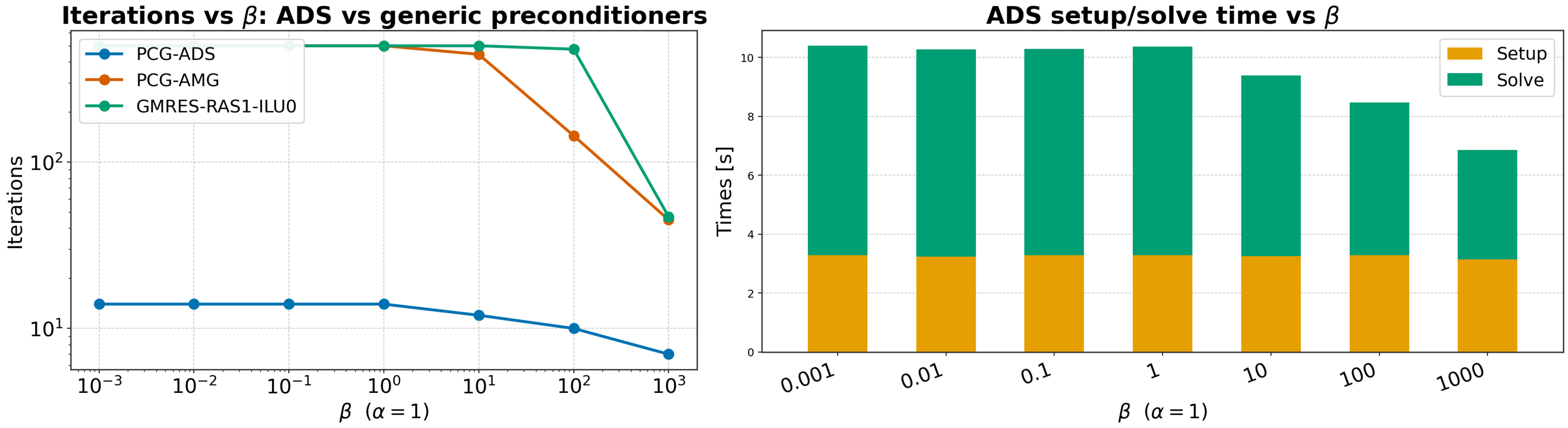
Definite grad-div problem on a \(64^3\) mesh (4 MPI ranks). Left: iteration count versus \(\beta\) (log-log) for ADS, BoomerAMG, and RAS(1)-ILU0. Right: stacked ADS setup/solve time versus \(\beta\).

ADS behaves exactly like its \(H(\mathrm{curl})\) counterpart: it is flat and robust (14 iterations in the div-dominated regime, easing to 7 when the mass term dominates), while BoomerAMG and RAS(1)-ILU0 hit the 500-iteration cap for small \(\beta\), recovering only once the mass term dominates. The ADS setup time is again independent of the coefficients, since the face-edge-node auxiliary hierarchy is built only from the discrete curl \(C\), the discrete gradient \(G\), and the coordinates; the solve time tracks the iteration count. The shared auxiliary-space machinery makes both solvers robust to the relative weight of the differential and mass terms, where generic algebraic preconditioners are not. (As in the Maxwell example, the comparison uses 4 MPI ranks because the bundled HYPRE’s overlapping-Schwarz setup aborts at higher rank counts on this \(64^3\) system.)